For many years I have been watching snooker, like sports. It has everything: the hypnotizing beauty of the intellectual game, the elegance of the blows of Ky and the psychological intensity of the competition. But there is one thing that I don’t like - his rating system .
Its main disadvantage is that it takes into account only the fact of tournament achievement without taking into account the "complexity" of matches. Such a deficiency is devoid of the Elo model , which monitors the players' “strength” and updates it depending on the results of the matches and the opponent's “strength”. However, it also does not fit perfectly: it is considered that all matches are played on an equal footing, and in snooker they are played until a certain number of frames won (games). To account for this fact, I considered another model, which I called EloBet .
This article examines the quality of Elo and EloBet models on the results of snooker matches. It is important to note that the main objectives are the assessment of the "strength" of the players and the creation of a "fair" rating, and not the construction of predictive models for obtaining benefits.

The current snooker rating is based on player achievements in tournaments with their different “weights”. Long ago, only World Championships were taken into account. After the appearance of many other competitions, a table of points was developed, which a player could earn, having reached a certain stage of the tournament. Now the rating looks like a "sliding" amount of prize money that the player earned during (approximately) the last two calendar years.
This system has two main advantages: it is simple (win a lot of money - go up in the ranking) and predictable (if you want to go up to a certain place - win a certain amount of money, other things being equal). The problem is that this method does not take into account the strength (skill, form) of rivals . The usual counter-argument is: "If a player has reached the late stage of a tournament, then he / she is by definition a strong player at the current moment" ("weak players do not win tournaments"). Sounds convincing enough. However, in snooker, as in any sport, the role of chance must be taken into account: if a player is "weaker", this does not mean that he / she can never win in a match against a player "stronger." It just happens less often than the opposite scenario. This is where the Elo model comes on the scene.
The idea of the Elo model is that each player is associated with a numerical rating. The assumption is introduced that the result of the game between two players can be predicted based on the difference in their ratings: higher values mean a higher probability of winning the “strong” player (with higher rating). Elo rating is based on the current "strength" , calculated on the basis of the results of matches with other players. This avoids the main drawback of the current official rating system. This approach also allows the player to update the rating during the tournament in order to respond numerically to his good performance.
Having practical experience with Elo rating, it seems to me that he should show himself well in snooker. However, there is one obstacle: it was created for competitions with a single type of match . Of course, there are variations to take into account the advantages of the home field in football and the first move in chess (both in the form of adding a fixed number of rating points to the player with the advantage). In snooker, matches are played in the "best of N" format: the player who wins the first wins. n= fracN+12 frames (batches). We will also call this format "to n victories. "
Intuitively, a victory in a match to 10 victories (the final of a serious tournament) should be given more difficult to a “weak” player than a victory in a match to 4 victories (the first round of current Home Nations tournaments). This is taken into account in the proposed EloBet model .
The idea of using Elo rating in snooker is by no means new. For example, there are the following works:
- Snooker Analyst uses an Elo-like (more like the Bradley – Terry model ) rating system. The idea is to update the rating based on the difference between the “real” and “expected” number of frames won. This approach raises questions. Of course, the greatest difference in the number of frames most likely demonstrates the larger difference in strength, but initially the player does not have such a task. In snooker, the goal is “just” to win the match, i.e. win a certain number of frames before the opponent.
- This discussion on the forum with the implementation of the basic model of Elo.
- This and this are real applications in amateur snooker.
- Perhaps there are other jobs that I missed. I would be very grateful for any information on this topic.
Overview
This article is intended for users of the R language who are interested in studying the Elo rating, and for snooker fans. All experiments are written with the idea of being reproducible. The code is hidden under the spoilers, has comments and uses the tidyverse packages, so it can be in itself interesting for users of R. It assumes the sequential execution of all the presented code. One file can be found here .
The article is organized as follows:
- The Model section describes the Elo and EloBet approaches with the implementation in R.
- The Experiment section describes the details and motivation of the calculation: what data and methodology is used (and why), and what results are obtained.
- The Study of EloBet ratings section contains the results of applying the EloBet model to real snooker data. It will be more interesting to snooker fans.
We will need the following initialization.
Initialization code# suppressPackageStartupMessages(library(dplyr)) library(tidyr) library(purrr) # library(ggplot2) # suppressPackageStartupMessages(library(comperank)) theme_set(theme_bw()) # . . set.seed(20180703)
Models
Both models are based on the following assumptions:
- There is a fixed set of players that must be ranked from the "strongest" (first place) to the "weakest" (last place).
- Ranking is done by associating a player. i numerically rated ri : A number representing the player’s "strength" (the larger the player’s stronger value).
- The greater the difference in ratings before a match, the less likely the victory of a “weak” player (with a lower rating).
- Ratings are updated after each match based on its result and ratings before it.
- A victory over a rival “stronger” must be accompanied by a higher rating increase than a victory over a rival “weaker”. With the defeat of the opposite is true.
Elo
Elo Model Code #' @details . #' `...` . #' #' @return , 1 ( `rating1`) #' 2 ( `rating2`). #' . elo_win_prob <- function(rating1, rating2, ksi = 400, ...) { norm_rating_diff <- (rating2 - rating1) / ksi 1 / (1 + 10^norm_rating_diff) } #' @return , #' `comperank::add_iterative_ratings()`. elo_fun_gen <- function(K, ksi = 400) { function(rating1, score1, rating2, score2) { comperank::elo(rating1, score1, rating2, score2, K = K, ksi = ksi)[1, ] } }
The Elo model updates the ratings according to the following procedure:
Calculation of the probability of a certain player's victory in a match (before it starts). The probability of winning one player (we will call him / her "first") with an identifier i and rated ri over another player ("second") with an identifier j and rated rj equals
Pr(ri,rj)= frac11+10(rj−ri)/400
With this approach, the calculation of probability obeys the third assumption.
Normalizing the difference by 400 is a mathematical way of saying which difference is considered “big”. This number can be replaced by the model parameter. xi However, this only affects the scatter of future ratings and is usually redundant. A value of 400 is fairly standard.
With a general approach, the probability of victory is L(rj−ri) where L(x) some strictly increasing function with values from 0 to 1. We will use the logistic curve. More complete research can be found in this article .
Match result calculation S . In the base model, it equals 1 in case of winning the first player (losing the second), 0.5 in the case of a tie, and 0 in the case of losing the first player (winning the second).
Rating update :
- delta=K cdot(S−Pr(ri,rj)) . This is the amount by which the ratings will change. She uses the coefficient K (the only parameter of the model). Lesser K (with equal probabilities) means less change in ratings - the model is more conservative, i.e. more victories are needed in order to “prove” a change in strength. On the other hand, more K means more "trust" in recent results than current ratings. Choosing the "optimal" K is a way to create a "good" rating system .
- r(new)i=ri+ delta , r(new)j=rj− delta .
Remarks :
- As can be seen from the update formulas, the sum of the ratings of all players considered does not change over time: the rating increases due to a decrease in the opponent’s rating
- Players without played matches are associated with an initial rating of 0. Or, values of 1500 or 1000 are usually used, but I do not see any other reason than psychological. Taking into account the previous remark, the use of zero means that the sum of all ratings is always zero, which is nice in its own way.
- It is necessary to play a certain number of matches in order for the rating to reflect the player’s “strength”. This presents a problem: new added players start with a rating of 0, which is certainly not the smallest among current players. In other words, "newbies" are considered "stronger" than some other players. You can try to deal with this by external rating update procedures when entering a new player.
Why does this algorithm make sense? In case of equality of ratings delta always equals 0.5 cdotK . Suppose, for example, that ri=0 and rj=400 . This means that the probability of winning the first player is equal to frac11+10 approx$0.090 i.e. he / she will win 1 match out of 11.
- In case of victory, he / she will receive an increase of approximately 0.909 cdotK That is more than in the case of equality of ratings.
- In case of defeat, he / she will receive a decrease of approximately 0.0909 cdotK That is less than in the case of equality of ratings.
This shows that the Elo model obeys the fifth assumption: a victory over an opponent "stronger" is accompanied by a higher rating increase than a victory over an opponent "weaker", and vice versa.
Of course, the Elo model has its own (rather high-level) practical features . However, the most important for our research is the following: it is assumed that all matches are held on an equal footing. This means that the distance of the match is not taken into account: a victory in a match to 4 victories is rewarded just as a victory in a match to 10 victories. Here the EloBet model comes on the scene.
EloBeta
EloBet model code #' @details . #' #' @return , 1 ( `rating1`) #' 2 ( `rating2`). `frames_to_win` #' . #' . elobeta_win_prob <- function(rating1, rating2, frames_to_win, ksi = 400, ...) { prob_frame <- elo_win_prob(rating1 = rating1, rating2 = rating2, ksi = ksi) # , `frames_to_win` # # (`prob_frame`). . pbeta(prob_frame, frames_to_win, frames_to_win) } #' @return : 1 / #' (), 0.5 0 / (). get_match_result <- function(score1, score2) { # () , . near_score <- dplyr::near(score1, score2) dplyr::if_else(near_score, 0.5, as.numeric(score1 > score2)) } #' @return , #' `add_iterative_ratings()`. elobeta_fun_gen <- function(K, ksi = 400) { function(rating1, score1, rating2, score2) { prob_win <- elobeta_win_prob( rating1 = rating1, rating2 = rating2, frames_to_win = pmax(score1, score2), ksi = ksi ) match_result <- get_match_result(score1, score2) delta <- K * (match_result - prob_win) c(rating1 + delta, rating2 - delta) } }
In the Elo model, the difference in ratings directly affects the probability of winning in the whole match. The main idea of the EloBet model is the direct influence of the rating difference on the probability of winning in one frame and explicit calculation of the player's probability of winning. n frames before the opponent .
The question remains: how to calculate this probability? It turns out that this is one of the oldest problems in the history of probability theory and has its own name - the problem of the division of bets (Problem of points). A very pleasant presentation can be found in this article . Using its notation, the desired probability equals:
P(n,n)= sum limits2n−1j=n2n−1 choosejpj(1−p)2n−1−j
Here P(n,n) - probability of the first player to win a match before n victories; p - the probability of his / her winning in one frame (the opponent has the probability 1−p ). With this approach, it is assumed that the results of the frame inside the match do not depend on each other . This may be questioned, but is a necessary assumption for this model.
Is there a faster way to calculate? It turns out the answer is yes. After a few hours of transformation of formulas, practical experiments and searches on the Internet, I found the following property of a regularized incomplete beta function. Ix(a,b) . Substituting m=k, n=2k−1 in this property and replacing k on n it turns out P(n,n)=Ip(n,n) .
This is also good news for R users, because Ip(n,n) can be calculated as pbeta(p, n, n) . Note : the general case of the probability of winning in n frames before the opponent wins m can also be calculated as Ip(n,m) and pbeta(p, n, m) respectively. This reveals the rich possibilities for updating the probability of winning during a match .
The procedure for updating ratings in the framework of the EloBet model is as follows (with well-known ratings ri and rj number of frames needed to win n and the result of the match S , as in the Elo model):
- The calculation of the probability of winning the first player in one frame : p=Pr(ri,rj)= frac11+10(rj−ri)/400 .
- The calculation of the probability of winning this player in the match : PrBeta(ri,rj)=Ip(n,n) . For example, if p equal to 0.4, then the probability of winning the match to 4 wins drops to 0.29, and in "to 18 wins" - to 0.11.
- Rating update :
- delta=K cdot(S−PrBeta(ri,rj)) .
- r(new)i=ri+ delta , r(new)j=rj− delta .
Note : because the difference in ratings directly affects the probability of winning in one frame, and not in the whole match, you should expect a lower optimal value of the coefficient K : part of the meaning delta comes from the reinforcing effect PrBeta(ri,rj) .
The idea of calculating the result of a match based on the probability of winning in one frame is not very new. On this website by François Labelle, you can find an online calculation of the probability of winning "best of N "match, along with other functions. I was glad to see that our calculation results are the same. However, I could not find any sources for the introduction of this approach in the Elo rating update procedure. As before, I would be very grateful for any information on this topic.
I was only able to find this article and the Elo system description on the backgammon game server (FIBS). There is also a Russian-language counterpart . Here, different duration of matches are taken into account by multiplying the difference of ratings by the square root of the distance of the match. However, it does not seem to have any theoretical justification.
Experiment
The experiment has several goals. Based on snooker match results:
- Determine the best coefficient values K for both models.
- Examine model stability in terms of predictive probability accuracy.
- To study the effect of using "invitation" tournaments on ratings.
- Create a "fair" ranking history for the season 2017/18 for all professional players.
Data
Experimental data generation code # "train", "validation" "test" split_cases <- function(n, props = c(0.5, 0.25, 0.25)) { breaks <- n * cumsum(head(props, -1)) / sum(props) id_vec <- findInterval(seq_len(n), breaks, left.open = TRUE) + 1 c("train", "validation", "test")[id_vec] } pro_players <- snooker_players %>% filter(status == "pro") # pro_matches_all <- snooker_matches %>% # filter(!walkover1, !walkover2) %>% # semi_join(y = pro_players, by = c(player1Id = "id")) %>% semi_join(y = pro_players, by = c(player2Id = "id")) %>% # 'season' left_join( y = snooker_events %>% select(id, season), by = c(eventId = "id") ) %>% # arrange(endDate) %>% # widecr transmute( game = seq_len(n()), player1 = player1Id, score1, player2 = player2Id, score2, matchId = id, endDate, eventId, season, # ("train", "validation" "test") # 50/25/25 matchType = split_cases(n()) ) %>% # widecr as_widecr() # (, # , Championship League). pro_matches_off <- pro_matches_all %>% anti_join( y = snooker_events %>% filter(type == "Invitational"), by = c(eventId = "id") ) # get_split <- . %>% count(matchType) %>% mutate(share = n / sum(n)) # 50/25/25 (train/validation/test) pro_matches_all %>% get_split() ## # A tibble: 3 x 3 ## matchType n share ## <chr> <int> <dbl> ## 1 test 1030 0.250 ## 2 train 2059 0.5 ## 3 validation 1029 0.250 # , # . , # __ __, `pro_matches_all`. # , __ # __. pro_matches_off %>% get_split() ## # A tibble: 3 x 3 ## matchType n share ## <chr> <int> <dbl> ## 1 test 820 0.225 ## 2 train 1810 0.497 ## 3 validation 1014 0.278 # K k_grid <- 1:100
We will use the comperank snooker data . The original source is snooker.org . The results are taken from the following matches:
- The match is played in the season 2016/17 or 2017/18 .
- The match is part of the "professional" snooker tournament , ie:
- It has the type "Invitational" ("Invitation"), "Qualifying" ("Qualifying") or "Ranking" ("Rating"). We will also distinguish between two sets of matches: "all matches" (from all tournament data) and "official matches" (excluding invitation tournaments). There are two reasons for this:
- In invitation tournaments, not all players have the opportunity to change their rating. This is not necessarily bad in the framework of Elo and EloBet models, but it has a "shade of injustice."
- There is a belief that the players "take seriously" only to the official rating matches. Note : most of the "Invitational" tournaments are part of the "Championship League", which I think is perceived by most players.
not very serious in the form of practice with the ability to make money. The presence of these tournaments may affect the rating. In addition to the "Championship League", there are other invitation tournaments: "2016 China Championship", both "Champion of Champions", both "Masters", "2017 Hong Kong Masters", "2017 World Games", "2017 Romanian Masters".
- Describes the traditional snooker (not 6 red or Power Snooker) between individual players (not teams).
- Both sexes can participate (not just men or women).
- Players of all ages can participate (not only seniors or "under 21").
- This is not "Shoot-Out", because These tournaments are stored differently in the snooker.org database.
- The match really took place : his result is the result of a real game involving both players.
- The match is held between two professionals . The list of professionals taken for the season 2017/18 (131 players). This decision seems the most controversial, because removal of matches involving amateurs "closes his eyes" to the defeat of professionals from amateurs. This leads to an unfair advantage of these players. It seems to me that such a decision is necessary to reduce the inflation of the rating , which will occur when taking into account matches with amateurs. Another approach is to study professionals and amateurs together, but this does not seem reasonable in this study. The defeat of a professional amateur is considered the loss of the opportunity to increase the rating.
The final number of matches used is 4118 for “all matches” and 3644 for “official matches” (62.9 and 55.6 per player, respectively).
Methodology
Experiment Function Code #' @param matches `longcr` `widecr` `matchType` #' ( : "train", "validation" "test"). #' @param test_type . #' #' ("") . , #' `game`. #' @param k_vec K . #' @param rate_fun_gen , K #' `add_iterative_ratings()`. #' @param get_win_prob #' (`rating1`, `rating2`) , #' (`frames_to_win`). ____: #' . #' @param initial_ratings #' `add_iterative_ratings()`. #' #' @details : #' - `matches` #' `game`. #' - `test_type`: #' - 1. #' - : 1 / #' (), 0.5 0 / (). #' - RMSE: , #' "" - . #' #' @return Tibble 'k' K 'goodness' #' RMSE. compute_goodness <- function(matches, test_type, k_vec, rate_fun_gen, get_win_prob, initial_ratings = 0) { cat("\n") map_dfr(k_vec, function(cur_k) { # cat(cur_k, " ") matches %>% arrange(game) %>% add_iterative_ratings( rate_fun = rate_fun_gen(cur_k), initial_ratings = initial_ratings ) %>% left_join(y = matches %>% select(game, matchType), by = "game") %>% filter(matchType %in% test_type) %>% mutate( # framesToWin = pmax(score1, score2), # 1 `framesToWin` winProb = get_win_prob( rating1 = rating1Before, rating2 = rating2Before, frames_to_win = framesToWin ), result = get_match_result(score1, score2), squareError = (result - winProb)^2 ) %>% summarise(goodness = sqrt(mean(squareError))) }) %>% mutate(k = k_vec) %>% select(k, goodness) } #' `compute_goodness()` compute_goodness_wrap <- function(matches_name, test_type, k_vec, rate_fun_gen_name, win_prob_fun_name, initial_ratings = 0) { matches_tbl <- get(matches_name) rate_fun_gen <- get(rate_fun_gen_name) get_win_prob <- get(win_prob_fun_name) compute_goodness( matches_tbl, test_type, k_vec, rate_fun_gen, get_win_prob, initial_ratings ) } #' #' #' @param test_type `test_type` ( ) #' `compute_goodness()`. #' @param rating_type ( ). #' @param data_type . #' @param k_vec,initial_ratings `compute_goodness()`. #' #' @details #' . #' , , #' : #' - "pro_matches_" + `< >` + `< >` . #' - `< >` + "_fun_gen" . #' - `< >` + "_win_prob" , #' . #' #' @return Tibble : #' - __testType__ <chr> : . #' - __ratingType__ <chr> : . #' - __dataType__ <chr> : . #' - __k__ <dbl/int> : K. #' - __goodness__ <dbl> : . do_experiment <- function(test_type = c("validation", "test"), rating_type = c("elo", "elobeta"), data_type = c("all", "off"), k_vec = k_grid, initial_ratings = 0) { crossing( testType = test_type, ratingType = rating_type, dataType = data_type ) %>% mutate( dataName = paste0("pro_matches_", testType, "_", dataType), kVec = rep(list(k_vec), n()), rateFunGenName = paste0(ratingType, "_fun_gen"), winProbFunName = paste0(ratingType, "_win_prob"), initialRatings = rep(list(initial_ratings), n()), experimentData = pmap( list(dataName, testType, kVec, rateFunGenName, winProbFunName, initialRatings), compute_goodness_wrap ) ) %>% unnest(experimentData) %>% select(testType, ratingType, dataType, k, goodness) }
"" K K=1,2,...,100 . , . :
- K :
- . , .
add_iterative_ratings() comperank . " ", .. . - , ( ) , . RMSE ( ) ( ). , RMSE=√1|T|∑t∈T(St−Pt)2 where T — , |T| — , St — , Pt — ( ). , " " .
- K RMSE . "" , RMSE K ( ). 0.5 ( "" 0.5) .
, : "train" (), "validation" () "test" (). , .. "train"/"validation" , "validation"/"test". 50/25/25 " ". " " " " . : 49.7/27.8/22.5. , , .
:
- : .
- : " " " " ( ". ").
- : "" ( "validation" RMSE "" "train" ) "" ( "test" RMSE "" "train" "validation" ).
results
pro_matches_validation_all <- pro_matches_all %>% filter(matchType != "test") pro_matches_validation_off <- pro_matches_off %>% filter(matchType != "test") pro_matches_test_all <- pro_matches_all pro_matches_test_off <- pro_matches_off
# experiment_tbl <- do_experiment()
plot_data <- experiment_tbl %>% unite(group, ratingType, dataType) %>% mutate( testType = recode( testType, validation = "", test = "" ), groupName = recode( group, elo_all = ", ", elo_off = ", . ", elobeta_all = ", ", elobeta_off = ", . " ), # groupName = factor(groupName, levels = unique(groupName)) ) compute_optimal_k <- . %>% group_by(testType, groupName) %>% slice(which.min(goodness)) %>% ungroup() compute_k_labels <- . %>% compute_optimal_k() %>% mutate(label = paste0("K = ", k)) %>% group_by(groupName) %>% # K , # . - # . mutate(hjust = - (k == max(k)) * 1.1 + 1.05) %>% ungroup() plot_experiment_results <- function(results_tbl) { ggplot(results_tbl) + geom_hline( yintercept = 0.5, colour = "#AA5555", size = 0.5, linetype = "dotted" ) + geom_line(aes(k, goodness, colour = testType)) + geom_vline( data = compute_optimal_k, mapping = aes(xintercept = k, colour = testType), linetype = "dashed", show.legend = FALSE ) + geom_text( data = compute_k_labels, mapping = aes(k, Inf, label = label, hjust = hjust), vjust = 1.2 ) + facet_wrap(~ groupName) + scale_colour_manual( values = c(`` = "#377EB8", `` = "#FF7F00"), guide = guide_legend(title = "", override.aes = list(size = 4)) ) + labs( x = " K", y = " (RMSE)", title = " ", subtitle = paste0( ' ( ) ', ' .\n', ' K ( ', '"") , .' ) ) + theme(title = element_text(size = 13), strip.text = element_text(size = 12)) } plot_experiment_results(plot_data)
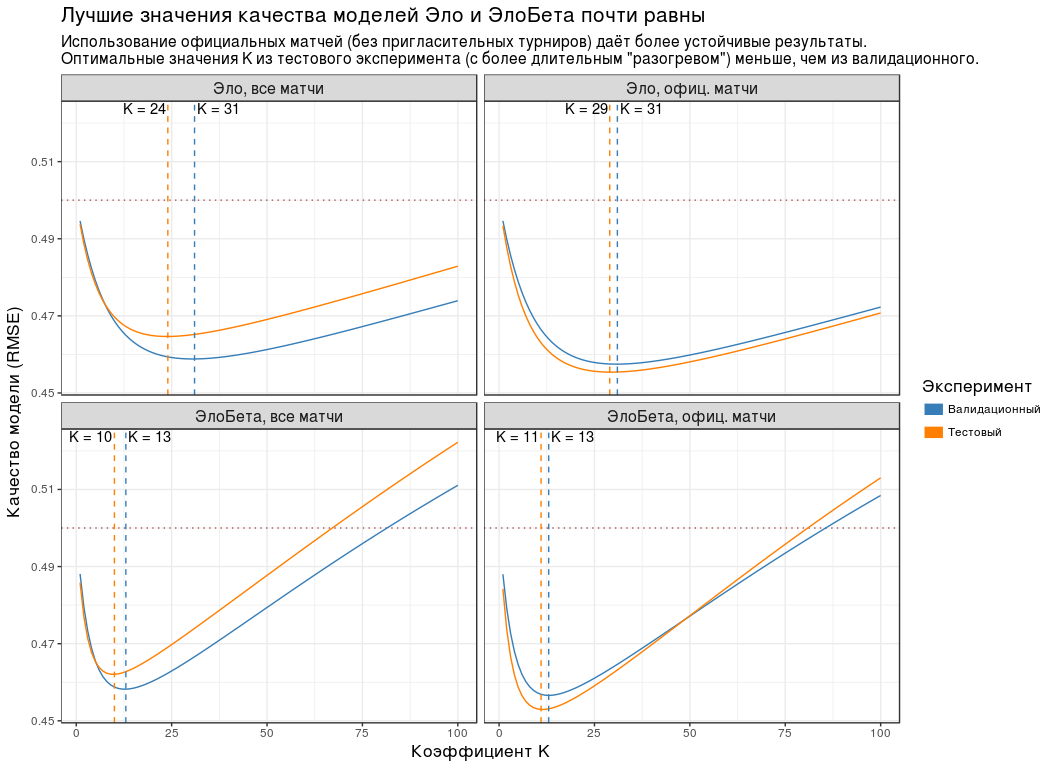
:
- , K , .
- ( "" "" ). , . - "Championship League": 3 .
- RMSE K . , RMSE K "" "". , " " .
- K ( "") , . "", .
- RMSE . 0.5. .
| Group | K | RMSE |
|---|
| , | 24 | 0.465 |
| , . | 29 | 0.455 |
| , | ten | 0.462 |
| , . | eleven | 0.453 |
Since , K " " ( ) 5: 30, — 10.
, K=30 K=10 . , n , .
" " ( K=10 ). - .
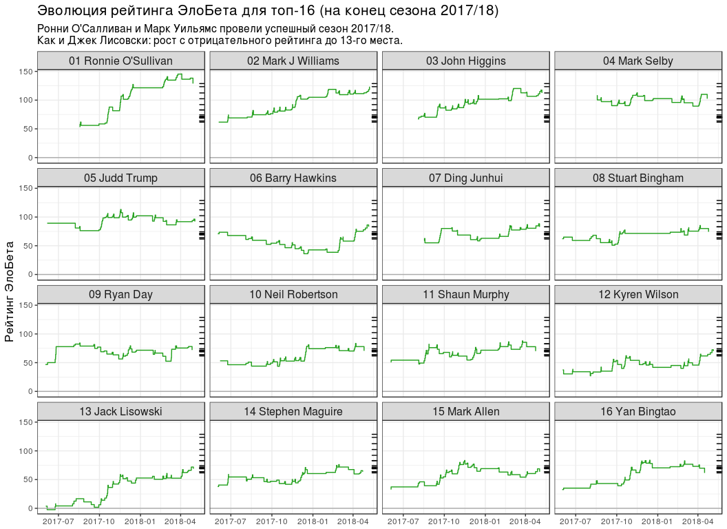
-16 2017/18
-16 2017/18 # gather_to_longcr <- function(tbl) { bind_rows( tbl %>% select(-matches("2")) %>% rename_all(funs(gsub("1", "", .))), tbl %>% select(-matches("1")) %>% rename_all(funs(gsub("2", "", .))) ) %>% arrange(game) } # K best_k <- experiment_tbl %>% filter(testType == "test", ratingType == "elobeta", dataType == "off") %>% slice(which.min(goodness)) %>% pull(k) #!!! "" , .. !!! best_k <- round(best_k / 5) * 5 # elobeta_ratings <- rate_iterative( pro_matches_test_off, elobeta_fun_gen(best_k), initial_ratings = 0 ) %>% rename(ratingEloBeta = rating_iterative) %>% arrange(desc(ratingEloBeta)) %>% left_join( y = snooker_players %>% select(id, playerName = name), by = c(player = "id") ) %>% mutate(rankEloBeta = order(ratingEloBeta, decreasing = TRUE)) %>% select(player, playerName, ratingEloBeta, rankEloBeta) elobeta_top16 <- elobeta_ratings %>% filter(rankEloBeta <= 16) %>% mutate( rankChr = formatC(rankEloBeta, width = 2, format = "d", flag = "0"), ratingEloBeta = round(ratingEloBeta, 1) ) official_ratings <- tibble( player = c( 5, 1, 237, 17, 12, 16, 224, 30, 68, 154, 97, 39, 85, 2, 202, 1260 ), rankOff = c( 2, 3, 4, 1, 5, 7, 6, 13, 16, 10, 8, 9, 26, 17, 12, 23 ), ratingOff = c( 905750, 878750, 751525, 1315275, 660250, 543225, 590525, 324587, 303862, 356125, 453875, 416250, 180862, 291025, 332450, 215125 ) )
-16 2017/18 ( snooker.org):
| Player | | | Officer | Officer | |
|---|
| Ronnie O'Sullivan | one | 128.8 | 2 | 905 750 | one |
| Mark J Williams | 2 | 123.4 | 3 | 878 750 | one |
| John Higgins | 3 | 112.5 | four | 751 525 | one |
| Mark Selby | four | 102.4 | one | 1 315 275 | -3 |
| Judd Trump | five | 92.2 | five | 660 250 | 0 |
| Barry Hawkins | 6 | 83.1 | 7 | 543 225 | one |
| Ding Junhui | 7 | 82.8 | 6 | 590 525 | -one |
| Stuart Bingham | eight | 74.3 | 13 | 324 587 | five |
| Ryan Day | 9 | 71.9 | sixteen | 303 862 | 7 |
| Neil Robertson | ten | 70.6 | ten | 356 125 | 0 |
| Shaun Murphy | eleven | 70.1 | eight | 453 875 | -3 |
| Kyren Wilson | 12 | 70.1 | 9 | 416 250 | -3 |
| Jack Lisowski | 13 | 68.8 | 26 | 180 862 | 13 |
| Stephen Maguire | 14 | 63.7 | 17 | 291 025 | 3 |
| Mark Allen | 15 | 63.7 | 12 | 332 450 | -3 |
| Yan Bingtao | sixteen | 61.6 | 23 | 215 125 | 7 |
:
- №1 3 . , , ( ).
- "" ( 13 ), ( 7 ).
- 5 . , 6 - WPBSA. , - "" . : , — .
- .
- ( №11), (№14) (№15) -16. "" (№26), (№23) (№17).
. , №16 (Yan Bingtao) №1 (Ronnie O'Sullivan) 0.404. 4 0.299, " 10 " — 0.197 18 — 0.125. , .
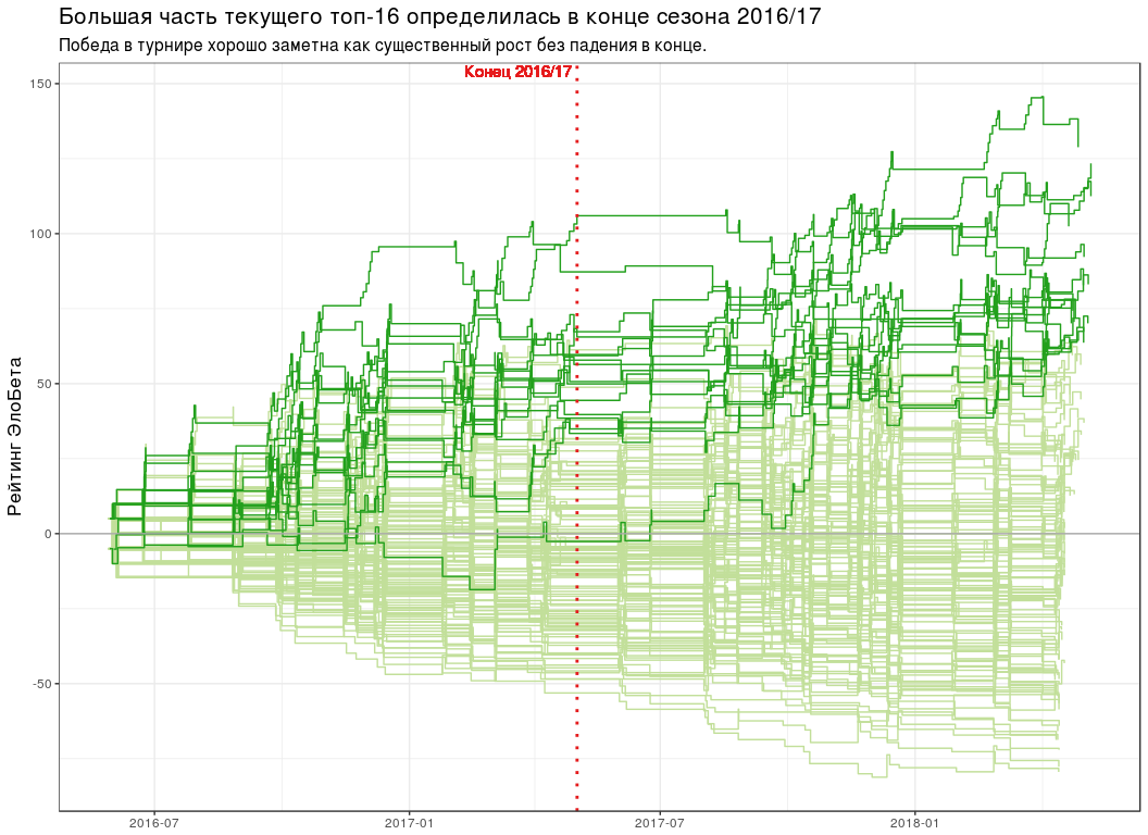
# seasons_break <- ISOdatetime(2017, 5, 2, 0, 0, 0, tz = "UTC") # elobeta_history <- pro_matches_test_off %>% add_iterative_ratings(elobeta_fun_gen(best_k), initial_ratings = 0) %>% gather_to_longcr() %>% left_join(y = pro_matches_test_off %>% select(game, endDate), by = "game") # plot_all_elobeta_history <- function(history_tbl) { history_tbl %>% mutate(isTop16 = player %in% elobeta_top16$player) %>% ggplot(aes(endDate, ratingAfter, group = player)) + geom_step(data = . %>% filter(!isTop16), colour = "#C2DF9A") + geom_step(data = . %>% filter(isTop16), colour = "#22A01C") + geom_hline(yintercept = 0, colour = "#AAAAAA") + geom_vline( xintercept = seasons_break, linetype = "dotted", colour = "#E41A1C", size = 1 ) + geom_text( x = seasons_break, y = Inf, label = " 2016/17", colour = "#E41A1C", hjust = 1.05, vjust = 1.2 ) + scale_x_datetime(date_labels = "%Y-%m") + labs( x = NULL, y = " ", title = paste0( " -16 2016/17" ), subtitle = paste0( " ", " ." ) ) + theme(title = element_text(size = 13)) } plot_all_elobeta_history(elobeta_history)
-16
-16 # top16_rating_evolution <- elobeta_history %>% # `inner_join` `elobeta_top16` inner_join(y = elobeta_top16 %>% select(-ratingEloBeta), by = "player") %>% # 2017/18 semi_join( y = pro_matches_test_off %>% filter(season == 2017), by = "game" ) %>% mutate(playerLabel = paste(rankChr, playerName)) # plot_top16_elobeta_history <- function(elobeta_history) { ggplot(elobeta_history) + geom_step(aes(endDate, ratingAfter, group = player), colour = "#22A01C") + geom_hline(yintercept = 0, colour = "#AAAAAA") + geom_rug( data = elobeta_top16, mapping = aes(y = ratingEloBeta), sides = "r" ) + facet_wrap(~ playerLabel, nrow = 4, ncol = 4) + scale_x_datetime(date_labels = "%Y-%m") + labs( x = NULL, y = " ", title = " -16 ( 2017/18)", subtitle = paste0( " ' 2017/18.\n", " : 13- ." ) ) + theme(title = element_text(size = 13), strip.text = element_text(size = 12)) } plot_top16_elobeta_history(top16_rating_evolution)
findings
- " " R :
pbeta(p, n, m) . - — "best of N " ( n ). .
- K=30 K=10 .
- :
sessionInfo() ## R version 3.4.4 (2018-03-15) ## Platform: x86_64-pc-linux-gnu (64-bit) ## Running under: Ubuntu 16.04.4 LTS ## ## Matrix products: default ## BLAS: /usr/lib/openblas-base/libblas.so.3 ## LAPACK: /usr/lib/libopenblasp-r0.2.18.so ## ## locale: ## [1] LC_CTYPE=ru_UA.UTF-8 LC_NUMERIC=C ## [3] LC_TIME=ru_UA.UTF-8 LC_COLLATE=ru_UA.UTF-8 ## [5] LC_MONETARY=ru_UA.UTF-8 LC_MESSAGES=ru_UA.UTF-8 ## [7] LC_PAPER=ru_UA.UTF-8 LC_NAME=C ## [9] LC_ADDRESS=C LC_TELEPHONE=C ## [11] LC_MEASUREMENT=ru_UA.UTF-8 LC_IDENTIFICATION=C ## ## attached base packages: ## [1] stats graphics grDevices utils datasets methods base ## ## other attached packages: ## [1] bindrcpp_0.2.2 comperank_0.1.0 comperes_0.2.0 ggplot2_2.2.1 ## [5] purrr_0.2.5 tidyr_0.8.1 dplyr_0.7.6 ## ## loaded via a namespace (and not attached): ## [1] Rcpp_0.12.17 knitr_1.20 bindr_0.1.1 magrittr_1.5 ## [5] munsell_0.5.0 tidyselect_0.2.4 colorspace_1.3-2 R6_2.2.2 ## [9] rlang_0.2.1 highr_0.7 plyr_1.8.4 stringr_1.3.1 ## [13] tools_3.4.4 grid_3.4.4 gtable_0.2.0 utf8_1.1.4 ## [17] cli_1.0.0 htmltools_0.3.6 lazyeval_0.2.1 yaml_2.1.19 ## [21] assertthat_0.2.0 rprojroot_1.3-2 digest_0.6.15 tibble_1.4.2 ## [25] crayon_1.3.4 glue_1.2.0 evaluate_0.10.1 rmarkdown_1.10 ## [29] labeling_0.3 stringi_1.2.3 compiler_3.4.4 pillar_1.2.3 ## [33] scales_0.5.0 backports_1.1.2 pkgconfig_2.0.1