GAN Learning Sustainability

The idea of ​​GAN was first published by Jan Goodfellow Generative Adversarial Nets, Goodfellow et alb 2014 , after which the GANs are among the best generative models.

Like any other generative model, the GAN task is to build a data model, and if more specifically learn how to generate samples from a distribution as close as possible to the distribution of data (there is usually a limited size data distribution in which we want to model).

GAN'y huge number of advantages, but they have one major drawback - they are very difficult to train.

Recently, a number of papers on the sustainability of GAN have been published:

• Gradient descent GAN optimization is locally stable, Vaishnavh Nagarajan, J. Zico Kolter, 2017
• The Numerics of GANs, Lars Mescheder et al, 2017

Inspired by their ideas, I did a little research.

I tried to make the text as simple as possible and if possible use only the simplest mathematics. Unfortunately, in order to justify why we can consider the properties of 2-dimensional vector fields, we have to dig a little towards the calculus of variations. But if these terms are not familiar to someone, you can safely move on to the consideration of 2-dimensional vector fields for different types of GANs.

We will now try to look under the hood of the training procedure and understand what is happening there.

GAN, the main problem

GANs consist of two neural networks: a discriminator and a generator. Generator - allows you to sample from some distribution (usually called the generator distribution). The discriminator receives samples from the original dataset and the generator at the entrance and learns to predict where this sample comes from (dataset or generator).

GAN scheme:



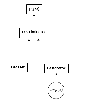
The GAN learning process is as follows:

1. Take n samples from dataset and m samples from generator.
2. We fix the generator weights and update the parameters of the discriminator. This is a common classification task. Only the need to train the discriminator to the convergence we do not have. And even more often it also interferes.
3. We fix the discriminator weights and make an update to the generator weights, so that the discriminator starts thinking that our samples are from the dataset and not from the generator.
4. Repeat 1-3 until the discriminator and the generator come to equilibrium (that is, neither one can "deceive" the other).

We will not consider in detail the process of learning GAN. On the Internet, and in particular, there are many articles explaining this process in detail.

We will be interested in something completely different. Namely, due to the fact that we have a competition of two neural networks, the task ceases to be a search for a minimum (maximum), and in some cases it turns into a search for a saddle point (i.e. at step 2 and 3 we are trying the same functionality maximize the discriminator parameters and minimize the generator parameters), and in the more common at steps 2 and 3 we can optimize completely different functionals. It is obvious that the minimax problem is a special case of optimization of different functionals - one functional is taken with different signs.

Let's look at it in the formulas. We assume that pd (x) is the distribution from where the dataset is sampled, pg (x) is the distribution of the generator, D (x) is the output from the discriminator.

When training a discriminator, we often maximize this functionality:

$$

$$J \ = \ \ int {p_d (x) log (D (x)) dx \ + \ \ int {p_g (x) log (1 \ - \ D (x)) dx}}$$

Gradient Vector:

$$

$$v = \ \ nabla_ \ theta J \ = \ int {\ frac {p_d (x)} {D (x)} \ nabla_ \ theta D (x) \ dx \ + \ \ int {\ frac {p_g (x )} {1 \ - \ D (x)} \ nabla_ \ theta D (x) dx}}$$

When training a generator, we maximize:

$$

$$I \ = \ - \ int {p_g (x) log (1 \ - \ D (x)) dx}$$

Gradient vector with:

$$

$$u \ = \ \ nabla_ \ varphi I \ = \ - \ int {{\ nabla_ \ varphi p} _g (x) log (1 \ - \ D (x)) dx}$$

In the future we will see that it is possible to replace the functionals respectively with:

$$

$$J \ = \ \ int {p_d (x) f_1 (D (x)) dx \ + \ \ int {p_g (x) f_2 (D (x)) dx}}$$

$$

$$I \ = \ \ int {p_g (x) f_3 (D (x)) dx}$$

Where $$$f_1, f_2, f_3$ selected by certain rules. By the way, Ian Goodfellow in his original article uses $$$f_1 and f_2$ as when learning the normal discriminator, and $$$f_3$ chooses such to improve gradients at the initial stage of training:

$$

$$f_1 \ left (x \ right) = log \ left (x \ right), \ f_2 \ left (x \ right) = log \ left (1 \ - \ x \ right), f_3 \ left (x \ right) = log \ left (x \ right)$$

At first glance, the task would seem to be very similar to the usual task of teaching gradient descent (ascent). Why, then, whoever has come across the GAN training, agree that it's damn hard?

The answer lies in the structure of the vector field, which we use to update the parameters of neural networks. In the case of the usual classification problem, we use only the vector of gradients, that is, the field is potential (the actually optimized functional is the potential of this vector field). And potential vector fields have some remarkable properties, one of which is the absence of closed curves. Ie in this field it is impossible to walk in circles. But when learning GAN, despite the fact that the vector fields for the generator and the discriminator are separately potential (this is gradient), the total vector field will not be potential. This means that there can be closed curves in this field, that is, we can walk in circles. And this is very, very bad.

The question arises, why did we manage to train the GAN quite successfully, can the field be irrotational (potential)? And if so, why is it so difficult?
Looking ahead, the field is unfortunately not potential, but it has a number of good properties. Unfortunately, the field is also very sensitive to the parameterization of neural networks (choice of activation functions, use of DropOut, BatchNormalization, etc.). But first things first.

“Gradient” GAN field

We will consider the functionals of learning GAN in the most general form:

$$

$$J \ = \ \ int {p_d (x) f_1 (D (x)) dx \ + \ \ int {p_g (x) f_2 (D (x)) dx}}$$

$$

$$I \ = \ \ int {p_g (x) f_3 (D (x)) dx}$$

We need to optimize both functional at the same time. If we assume that D (x) and pg (x) are absolutely flexible functions, i.e. we can take any number at any point, regardless of other points. That known fact from the variational calculus - the function needs to be changed in the direction of the variational derivative of this functional (in general, a complete analogue of the gradient lift).

We write the variational derivative:

$$

$$\ frac {\ partial J} {\ partial D (x)} = p_d (x) f_1 '(D (x)) \ + \ p_g (x) f_2' (D (x))$$

$$

$$\ frac {\ partial I} {\ partial p_g (x)} = f_3 (D (x))$$

We will consider only the first function (for the discriminator), for the second, everything will be the same.

But considering that in fact we can change the function only in the set of functions that are represented by our neural network, we will write:

$$$$ display $$ ∆D (x) = \ frac {\ partial D (x)} {\ partial θ_j} ∆θ_j $$ display $$

changes in network parameters, in general, the usual gradient descent (ascent):

$$$$ display $$ ∆θj = \ frac {\ partial J} {\ partial θ_j} μ $$ display $$

µ is the learning rate. Well, the derivative of the network parameters:

$$

$$\ frac {\ partial J} {\ partial \ theta_j} = \ int {\ frac {\ partial J} {\ partial D (y)} \ frac {\ partial D (y)} {\ partial \ theta_j} dy }$$

And now we collect everything together:

$$

$$∆D (x) = \ sum_ {j} {\ frac {\ partial D (x)} {\ partial \ theta_j} \ int {\ frac {\ partial J} {\ partial D (y)} \ frac { \ partial D (y)} {\ partial \ theta_j} dy} \ mu \ = \ mu \ int \ frac {\ partial J} {\ partial D (y)}} \ sum_ {j} {\ frac {\ partial D (x)} {\ partial \ theta_j} \ frac {\ partial D (x)} {\ partial \ theta_j} dy \ = \} \ mu \ int {\ frac {\ partial J} {\ partial D (y )} K_ \ theta (x, y) dy}$$

Where: $$$K_ \ theta (x, y) \ = \ sum_ {j} {\ frac {\ partial D (x)} {\ partial \ theta_j} \ frac {\ partial D (x)} {\ partial \ theta_j} \ }$

I have never met this function in the machine learning literature, so I will call it the parametric core of the system.

Well, or if we go to continuous time steps (from difference equations to differential ones), we get:

$$

$$\ frac {d} {dt} D (x) \ = \ \ int {\ frac {\ partial J} {\ partial D (y)} K_ \ theta (x, y) dy}$$

This equation shows the internal connection of the original field (point-to-point for the discriminator) and the parametrization of the neural network. We obtain a completely analogous equation for the generator.

Given that K (x, y) (parametric core) is a positive definite function (well, how can it be represented as a scalar product of gradients at corresponding points), we can conclude that any changes to the learning functions (discriminator and generator) belong to Hilbert space generated by the kernel, i.e. K (x, y). Is it interesting to get any meaningful results here? But we will not look at that side for now, but look at the other.

As can be seen, the stability of the GAN is determined by two components: the variational derivatives of the functionals and the parameterization of the neural network. Our task is to see how this field behaves point-by-point, that is, if our network can represent absolutely any function. The task turns into an analysis of a two-dimensional vector field. And this, I think, is in our power.

Resilience

So, we consider the following vector field:

$$

$$\ frac {d} {dt} D (x) = \ \ frac {\ partial J} {\ partial D (x)}$$

$$

$$\ frac {d} {dt} p_g (x) = \ \ frac {\ partial I} {\ partial p_g (x)}$$

It is obvious that these equations can be considered for only one point x, taking into account how our variational derivatives look like:

$$

$$\ frac {d} {dt} D = \ p_df_1 ^ \ prime (D) \ + \ p_gf_2 ^ \ prime (D)$$

$$

$$\ frac {d} {dt} p_g \ = \ f_3 (D)$$

The first requirement for this system of equations is that the right-hand side must go to 0 when:
$$$p_d = p_g$

Otherwise, we will try to train a model that obviously will not converge to the correct solution. Those. D must be a solution to the following equation:

$$

$$f_1 ^ \ prime (D) \ + \ f_2 ^ \ prime (D) \ = \ 0$$

Denote this solution as $$$D0$ .

Given the fact that pg (x) is the probability density, we can add any number to the right-hand side without disturbing the derivatives. In order to provide 0 of the right-hand side at the desired point, we subtract the value in m. $$$D0$ (it is necessary to do this if we want to consider pg point by point - the transition from the field parametrized by probability densities to free fields).

As a result, we get the following field:

$$

$$\ frac {d} {dt} D = \ p_df_1 ^ \ prime (D) \ + \ p_gf_2 ^ \ prime (D)$$

$$

$$\ frac {d} {dt} p_g \ = \ f_3 (D) \ - \ f (D0)$$

From this moment on we will study the points of rest and the stability of fields of precisely this kind.
We can study two types of stability: local (in the neighborhood of a point of rest) and global (using the method of Lyapunov functions).

To study local stability, it is necessary to calculate the Jacobi field matrix.
In order for the field to be locally “stable” it is necessary that the eigenvalues ​​have a negative real part.

Different types of gan

1. Classic GAN

   
   
   In the classic GAN, we use the usual logloss:
   

   $$

   $$J \ = \ \ int {p_d (x) log (D (x)) dx \ + \ \ int {p_g (x) log (1 \ - \ D (x)) dx}}$$
   
   To train a discriminator, it is necessary to maximize it, for a generator - to minimize it. In this case, the field will look like this:
   

   $$

   $$\ frac {d} {dt} D = \ \ frac {p_d} {D} \ - \ \ frac {p_g} {1-D}$$
   
   

   $$

   $$\ frac {d} {dt} p_g \ = \ -log (1-D) \ + \ log (\ frac {1} {2})$$
   
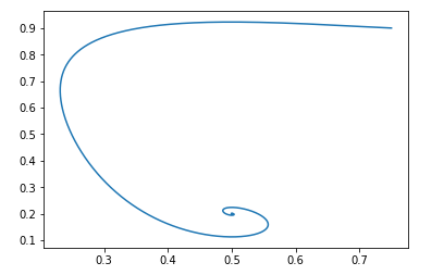
   Let's see how the parameters (pg and D) in this field will evolve. To do this, use such a simple Python script:
   
   
   Script

   def get_v(d, pg, pd): vd = pd/d - pg/(1.-d) vpg = -np.log(1.-d) + np.log(0.5) return vd, vpg d = 0.75 pg = 0.9 pd = 0.2 d_hist = [] pg_hist = [] lr = 1e-3 n_iter = 100000 for i in range(n_iter): d_hist.append(d) pg_hist.append(pg) vd, vpg = get_v(d, pg, pd) d = d + lr*vd pg = pg + lr*vpg plt.plot(d_hist, pg_hist, '-') plt.show() 

   
   
   
   For the starting point $$$p_g = 0.9, D = 0.25$ it will look like this:
   
   
   
   The rest point of such a field will be: pg = pd and D = 0.5
   
   It is easy to verify that the real parts of the eigenvalues ​​of the Jacobi matrix are negative, that is, the field is locally stable.
   We will not deal with evidence of global sustainability. But if it is very interesting, you can play around with the Python script and make sure that the field is stable for any valid initial values.

2. Modification by Jan Goodfellow

   
   We have already discussed above that Ian Goodfellow in the original article used a slightly modified version of the GAN. For his version, the functions were as follows:
   

   $$

   $$f_1 \ left (x \ right) = log \ left (x \ right), \ f_2 \ left (x \ right) = log \ left (1 \ - \ x \ right), f_3 \ left (x \ right) = log \ left (x \ right)$$
   
   The field will look like this:
   

   $$

   $$\ frac {d} {dt} D = \ \ frac {p_d} {D} \ - \ \ frac {p_g} {1-D}$$
   
   

   $$

   $$\ frac {d} {dt} p_g \ = \ log (D) \ - \ log (\ frac {1} {2})$$
   
   The Python script will be the same, only the function of the field is different:
   
   
   Script

    def get_v(d, pg, pd): vd = pd/d - pg/(1.-d) vpg = np.log(d) - np.log(0.5) return vd, vpg d = 0.75 pg = 0.9 pd = 0.2 d_hist = [] pg_hist = [] lr = 1e-3 n_iter = 100000 for i in range(n_iter): d_hist.append(d) pg_hist.append(pg) vd, vpg = get_v(d, pg, pd) d = d + lr*vd pg = pg + lr*vpg plt.plot(d_hist, pg_hist, '-') plt.show() 

   
   
   
   And with the same initial data, the picture looks like this:
   
   
   
   And again, it is easy to verify that the field will be locally stable.
   That is, from the point of view of convergence, such a modification does not degrade the properties of the GAN, but it has its advantages from the point of view of learning neural networks.

3. Wasserstein gan

   
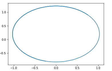
   Let's look at another popular type of GAN. Optimized functionality looks like this:
   

   $$

   $$J \ = \ \ int {p_d (x) D (x) dx \ - \} \ int {p_g (x) D (x) dx}$$
   
   Where D belongs to the class of 1-Lipschitz functions in x.
   We want to maximize it in D and minimize in pg.
   
   Obviously, in this case: $$$f_1 \ left (x \ right) = x, \ f_2 \ left (x \ right) = - x, \ f_3 \ left (x \ right) = x$
   
   And the field will look like this:
   

   $$

   $$\ frac {d} {dt} D = \ p_d \ - {\ p} _g \ $$
   
   

   $$

   $$\ frac {d} {dt} p_g \ = \ D$$
   
   This field easily guesses a circle centered at $$$p_g = p_d, D = 0$ .
   That is, if we go around this field, we will walk forever in a circle.
   
   Here is an example of the trajectory in this field:
   
   
   
   The question arises, why is it then possible to train this type of GAN? The answer is very simple - this analysis does not take into account the fact that 1-Lipschitz property D. That is, we cannot take arbitrary functions. By the way, this is in good agreement with the results of the authors ... of the article. To avoid walking in a circle, they recommend to train the discriminator to convergence: Wasserstein GAN

4. New GAN Options

   
   Feature selection $$$f_1, f_2 and f_3$ You can create different variants of GAN. The main requirement for these functions is to ensure the presence of the "correct" rest point and the stability of this point (preferably global, but at least local). I give the reader the opportunity to deduce the restrictions on the functions f1, f2 and f3 necessary for local stability. It is easy - it suffices to consider a quadratic equation for the eigenvalues ​​of the Jacobi matrix.
   
   I will give an example of such a GAN:
   

   $$

   $$f_1 (x) \ = \ -0.5x ^ 2, \ f_2 (x) \ = \ x, \ f_3 (x) \ = \ -x$$
   
   Again, I suggest that the reader build the field of this GAN himself and prove its stability. (By the way, this is one of the few fields for which the proof of global sustainability is elementary - it is enough to choose the Lyapunov function distance to the point of rest). Just need to take into account that the point of rest D = 1.

Conclusion and further research

From the above analysis, it is clear that all classic GANs (with the exception of the Wassertein GAN, which has its own ways of improving stability) have “good” fields. Those. following these fields has a single repentance point in which the distribution of the generator is equal to the distribution of the data.

Why then is learning GAN such a difficult task. The answer is simple - parametrization of neural networks. With the "bad" parameterization, we can also go for a walk in circles. For example, in my experiments show that, for example, using BatchNormalization in any of the networks immediately turns the field into a closed one. And Relu activation works best.

Unfortunately, at the moment there is not a single way to theoretically check what elements of a neural network change the field. It will prove to me promising to investigate the properties of the system’s parametric core - $$$K_ \ theta (x, y)$ .

I also wanted to tell you about the ways of regularizing the GAN fields and a look from the position of two-dimensional fields on this. Consider the Reinforcement Learning algorithms from this position. And much more. But unfortunately, the article and so it turned out too big, so about this as some other time.