Pitch-tracking, or determining the pitch frequency in speech, using the examples of Praat, YAAPT and YIN algorithms

In the field of emotion recognition, the voice is the second most important source of emotional data after a face. The voice can be characterized by several parameters. The pitch of the voice is one of the main characteristics, but in the field of acoustic technology it is more correct to call this parameter the pitch frequency.

The pitch frequency is directly related to what we call intonation. And intonation, for example, is associated with emotional and expressive characteristics of the voice.

However, determining the pitch frequency is not an entirely trivial task with interesting nuances. In this article, we will discuss the features of the algorithms for its definition and compare the existing solutions with examples of specific audio recordings.

Introduction

To begin with, let us remember what, in essence, is the frequency of the fundamental tone and in what tasks it may be needed. The pitch frequency , which is also designated as CHOT, Fundamental Frequency or F0 is the frequency of the oscillation of the vocal cords when pronouncing tonal sounds (voiced). When uttering non-tones (unvoiced), for example, speaking in a whisper or pronouncing hissing and whistling sounds, the ligaments do not fluctuate, which means that this characteristic is not relevant for them.

* Please note that the division into tonal and non-tonal sounds is not equivalent to the division into vowels and consonants.

The pitch frequency variability is quite large, and it can be very different not only between people (for lower average male voices, the frequency is 70-200 Hz, and for female voices it can reach 400 Hz), but also for one person, especially in emotional speech .

Determining the pitch frequency is used to solve a wide range of tasks:

• Recognition of emotions, as we said above;
• Sex determination;
• In solving the problem of segmentation of audio with several voices or division of speech into phrases;
• In medicine, to determine the pathological characteristics of the voice (for example, using acoustic parameters of Jitter and Shimmer). For example, the definition of signs of Parkinson's disease [ 1 ]. Jitter and Shimmer can also be used to recognize emotions [ 2 ].

However, there are a number of difficulties in determining F0. For example, you can often confuse F0 with harmonics, which can lead to so-called pitch doubling / pitch halving effects [ 3 ]. And in the audio recording of poor quality, F0 is quite difficult to calculate, since the desired peak at low frequencies almost disappears.

By the way, do you remember the story about Laurel and Yanny ? Differences in what words people hear when listening to the same audio recordings, have arisen precisely because of the difference in the perception of F0, which is influenced by many factors: the age of the listener, the degree of fatigue, the playback device. So, when listening to the recording in speakers with high-quality reproduction of low frequencies, you will hear Laurel, and in audio systems where low frequencies are reproduced poorly, Yanny. The transition effect can be seen on one device, for example, here . And in this article , the neural network acts as a listener. In another article you can read, as explained by the phenomenon of Yanny / Laurel from the standpoint of speech formation.

Since a detailed analysis of all the methods for determining F0 would be too voluminous, the article is an overview and can help orient oneself in the topic.

Methods for determining F0

Methods for determining F0 can be divided into three categories: based on the temporal dynamics of the signal, or time-domain; based on the frequency structure, or frequency-domain, as well as combined methods. We suggest to get acquainted with the review article on the topic, where the designated methods of extracting F0 are described in detail.

Note that any of the algorithms discussed consists of 3 basic steps:

Preprocessing (signal filtering, splitting it into frames)
Search for possible values ​​of F0 (candidates)
Tracking is the choice of the most probable trajectory F0 (since for each moment in time we have several competing candidates, we need to find the most probable track among them)

Time domain

We outline a few general points. Before applying the time-domain methods, the signal is pre-filtered, leaving only the low frequencies. Thresholds are set - the minimum and maximum frequencies, for example, from 75 to 500 Hz. The definition of F0 is made only for sections with harmonic speech, since for pauses or noise sounds this is not only meaningless, but it can introduce errors into neighboring frames when applying interpolation and / or smoothing. The frame length is chosen so that it contains at least three periods.

The main method, on the basis of which subsequently appeared a whole family of algorithms - autocorrelation. The approach is quite simple - it is necessary to calculate the autocorrelation function and take its first maximum. It will display the most pronounced frequency component in the signal. What can be the difficulty in the case of using autocorrelation, and why is it not always the first maximum will correspond to the desired frequency? Even in close to ideal conditions on high quality recordings, the method may be mistaken due to the complex structure of the signal. In conditions close to real, where, among other things, we may face the disappearance of the necessary peak on noisy recordings or recordings of initially poor quality, the number of errors increases sharply.

Despite the errors, the autocorrelation method is quite convenient and attractive with its basic simplicity and logic, therefore, it is used as the basis for many algorithms, including YIN (Yin). Even the name of the algorithm refers us to the balance between convenience and inaccuracy of the autocorrelation method: “From the“ yin ”“ and “from the interplay between autocorrelation and cancellation that it includes.” [ 4 ]

The creators of YIN tried to correct the weak points of the auto-correlation approach. The first change is the use of the Cumulative Mean Normalized Difference function, which should reduce the sensitivity to amplitude modulations, making the peaks more pronounced:

\ begin {equation}
d'_t (\ tau) =
\ begin {cases}
1, & \ tau = 0 \\
d_t (\ tau) \ bigg / \ bigg [\ frac {1} {\ tau} \ sum \ limits_ {j = 1} ^ {\ tau} d_t (j) \ bigg], & \ text {otherwise}
\ end {cases}
\ end {equation}
YIN also tries to avoid errors that occur when the length of the window function is not completely divided by the oscillation period. Parabolic interpolation of the minimum is used for this. At the last audio processing step, the Best Local Estimate function is performed to prevent sharp jumps in values ​​(good or bad - a moot point).

Frequency-domain

If we talk about the frequency domain, then the harmonic structure of the signal, that is, the presence of spectral peaks at frequencies multiple of F0, comes to the fore. The “collapse” of this periodic pattern to a clear peak can be made by means of a cepstral analysis. Kepstrum - Fourier transform of the logarithm of the power spectrum; the cepstral peak corresponds to the most periodic component of the spectrum (one can read about it here and here ).

Hybrid methods for determining F0

The following algorithm, which is worth dwelling on in more detail, has the talking name YAAPT - Yet Another Algorithm of Pitch Tracking - and in fact is a hybrid, because it uses both frequency and time information. A full description is in the article , here we describe only the main stages.


Figure 1. YAAPTalgo algorithm diagram ( reference ) .

YAAPT consists of several basic steps, the first of which is preprocessing. At this stage, the values ​​of the original signal are squared, get the second version of the signal. This step has the same goal as the Cumulative Mean Normalized Difference Function in YIN - to enhance and restore “erased” autocorrelation peaks. Both versions of the signal filter - usually take the range of 50-1500 Hz, sometimes 50-900 Hz.

Then, the base path F0 is calculated from the spectrum of the converted signal. F0 candidates are determined using the Spectral Harmonics Correlation (SHC) function.

\ begin {equation}
SHC (t, f) = \ sum \ limits_ {f '= - WL / 2} ^ {WL / 2} \ prod \ limits_ {r = 1} ^ {NH + 1} S (t, rf + f')
\ end {equation}
where S (t, f) is the magnitude spectrum for frame t and frequency f, WL is the window length in Hz, NH is the number of harmonics (the authors recommend using the first three harmonics). Also, spectral power is used to determine voiced-unvoiced frames, after which the most optimal trajectory is sought, taking into account the possibility of pitch doubling / pitch halving [ 3 , Section II, C].

Further, both for the initial signal and for the transformed one, the candidates for F0 are determined, and instead of the autocorrelation function, the Normalized Cross Correlation (NCCF) is used here.

\ begin {equation}
NCCF (m) = \ frac {\ sum \ limits_ {n = 0} ^ {Nm-1} x (n) * x (n + m)} {\ sqrt {\ sum \ limits_ {n = 0} ^ { Nm-1} x ^ 2 (n) * \ sum \ limits_ {n = 0} ^ {Nm-1} x ^ 2 (n + m)}} \ text {,} \ hspace {0.3cm} 0 <m <M_ {0}
\ end {equation}
The next stage is the evaluation of all possible candidates and the calculation of their significance, or weight (merit). The weight of candidates received from an audio signal depends not only on the amplitude of the NCCF peak, but also on their proximity to the F0 trajectory determined from the spectrum. That is, the frequency domain is considered, though rough in terms of accuracy, but stable [ 3 , Section II, D].

Then, for all pairs of the remaining candidates, the Transition Cost matrix is ​​calculated - the transition costs, which ultimately find the optimal trajectory [ 3 , Section II, E].

Examples

Now apply all the above algorithms to specific audio recordings. As a starting point, we will use Praat - a tool that is fundamental to many speech researchers. And then in Python we will look at the implementation of YIN and YAAPT and compare the results obtained.

You can use any available audio as audio material. We took several passages from our RAMAS database - a multimodal dataset created with the participation of the VGIK actors. You can also use material from other open bases, such as LibriSpeech or RAVDESS .

For illustrative example, we took excerpts from several recordings with male and female voices, both neutral and emotionally-colored, and for clarity, we combined them into one recording . Let's look at our signal, its spectrogram, intensity (orange), and F0 (blue). In Praat, this can be done using Ctrl + O (Open - Read from file) and then the View & Edit buttons.


Figure 2. Spectrogram, intensity (orange), F0 (blue) in Praat.

The audio shows quite clearly that with emotional speech, the pitch of the voice increases in both men and women. At the same time, F0 for emotional male speech can be compared with F0 of a female voice.

Tracking

In the Praat menu, select the Analyze periodicity - to Pitch (ac) tab, that is, the definition of F0 using autocorrelation. A window for specifying parameters will appear, in which there is an opportunity to set 3 parameters for determining candidates for F0 and another 6 parameters for the path search algorithm (path-finder), which builds the most probable trajectory F0 among all candidates.


A detailed description of the algorithm can be found in the article in 1993.

The result of the tracker (path-finder) operation can be viewed by clicking OK and then viewing (View & Edit) the resulting Pitch file. It can be seen that in addition to the chosen trajectory there were still quite significant candidates with a frequency below.


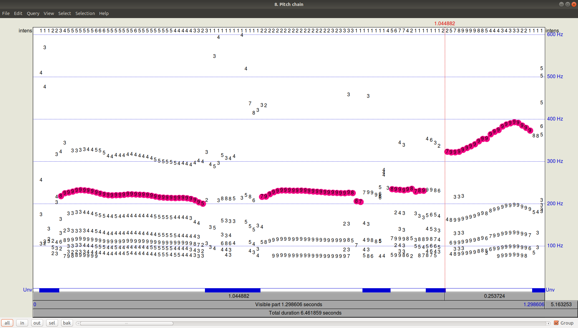Figure 3. PitchPath for the first 1.3 seconds of audio recording.

And what about Python?

Let's take two libraries that offer pitch-tracking - aubio , in which the default algorithm is YIN, and the AMFM_decompsition library, in which there is a realization of the YAAPT algorithm. Paste the F0 values ​​from Praat into the separate file ( PraatPitch.txt file) (you can do this manually: select the audio file, click View & Edit, select the entire file and select Pitch-Pitch listing in the top menu).

Now compare the results for all three algorithms (YIN, YAAPT, Praat).




Figure 4. Comparison of the operation of the algorithms YIN, YAAPT and Praat.

We see that with the default settings, YIN is quite distracting, getting a very flat trajectory with understated values ​​for Praat and completely losing transitions between a male and a female voice, as well as between emotional and non-emotional speech.

YAAPT stabbed a very high tone with emotional female speech, but in general, clearly managed better. Due to its specific features, YAAPT works better - it is impossible to answer right away, of course, but we can assume that the role is played by receiving candidates from three sources and a more scrupulous calculation of their weight than in YIN.

Conclusion

Since the question of determining the pitch frequency (F0) in one form or another is confronted by almost everyone who works with sound, there are many ways to solve it. The question of the required accuracy and the specifics of the audio material in each particular case determine how carefully it is necessary to select the parameters, or otherwise you can limit yourself to a basic solution like YAAPT. Taking Praat as a benchmark for speech processing (a huge number of researchers still use it), we can conclude that YAAPT is more reliable and more accurate than YIN as a first approximation, although our example turned out to be more complicated for it.

Author: Eva Kazimirova , Researcher, Neurodata Lab, Speech Processing Specialist.

Offtop : Did you like the article? In fact, we have a lot of similar interesting tasks on ML, mathematics and programming, and we need brains. Are you interested in this? Come to us! E-mail: hr@neurodatalab.com