Learn OpenGL. Lesson 5.6 - Parallax Mapping

Parallax mapping

The Parallax Mapping texturing technique is somewhat similar in its effect to Normal Mapping ', but based on a different principle. The similarity is that, like Normal Mapping, this technique significantly increases the visual complexity and detail of the surface with the applied texture at the same time creating a plausible illusion of the presence of height differences on the surface. Parallax Mapping works great in conjunction with Normal Mapping to create very reliable results: the technique described conveys the relief effect much better than Normal Mapping, and Normal Mapping complements it for a realistic simulation of dynamic lighting. Parallax Mapping can hardly be considered a technique directly related to the methods of imitation of lighting, but still I chose this section to consider it, since the method is a logical development of the ideas of Normal Mapping. Also note that to parse this article requires a good understanding of the operation of the Normal Mapping, especially the concept of tangent space or tangent space .


Parallax Mapping refers to the Displacement Mapping or relief texturing family of techniques that displace geometry vertices based on values ​​stored in special texture maps. For example, imagine a plane composed of about a thousand vertices. Each of them can be shifted according to the value read from the texture, which is the height of the plane at the given point. This texture, containing the height values ​​in each texel, is called the height map . An example of such a map, obtained on the basis of the geometric characteristics of the surface of brickwork, is the following image:


By sampling from this map and displacing each vertex according to the height value, it is possible to obtain from a perfect plane a convex surface that repeats the geometric parameters of the original surface. So, taking a plane with a sufficient number of vertices and applying the height map from the example, you can get the following result:


The described approach is simple and easy to implement, but requires a high density of vertices in the object being processed, otherwise the result of the shift will be too rough. And if on each flat surface you start to release over a thousand or more vertices, then very soon we will simply not have time to render everything we need. Maybe there is an algorithm that allows to qualitatively simulate the quality of the naive Displacement Mapping algorithm, but at the same time without requiring such costs for geometry? If you are standing, sit down, since there are actually only six vertices (two triangles) in the image above! The relief of the brickwork is perfectly simulated thanks to the use of Parallax Mapping, a relief texturing technique that does not require a multitude of vertices for a plausible transfer of the surface relief, and, like Normal Mapping, which uses an original approach to deceive the eye of the observer.

The main idea of ​​the implementation is to distort the texture coordinates for the current fragment based on the direction of the sight and the height map data so as to create the illusion that this fragment belongs to a surface area lying higher or lower than it actually is. For a better understanding of the principle, look at the diagram of our example with bricks:

Here, the coarse red line represents the values ​​from the height map, reflecting the geometric characteristics of the simulated surface of the brickwork. Vector $$$\ color {orange} {\ bar {V}}$ is the direction from the surface to the observer ( viewDir ). If the plane were really a relief, the observer would see a point on the surface $$$\ color {blue} B$ . However, in fact we have an ideal plane and the ray in the direction of gaze intersects the plane at the point $$$\ color {green} A$ which is obvious. The task of Parallax Mapping to shift the texture coordinates at a point $$$\ color {green} A$ so that they become identical to the coordinates corresponding to the point $$$\ color {blue} B$ . Further for the current fragment (corresponds to the point $$$\ color {green} A$ ) we use the obtained coordinates of the point $$$\ color {blue} B$ texture samples are required for all, which creates the illusion that the observer sees the point $$$\ color {blue} B$ .

The main difficulty lies in how to calculate the texture coordinates of a point $$$\ color {blue} B$ being at the point $$$\ color {green} A$ . Parallax Mapping offers an approximate solution, applying a simple scaling of the direction vector from the surface $$$\ color {orange} {\ bar {V}}$ to the observer by the magnitude of the height for the fragment $$$\ color {green} A$ . Those. just change the length $$$\ color {orange} {\ bar {V}}$ so that it matches the sample size from the height map $$$\ color {green} {H (A)}$ corresponding to the fragment $$$\ color {green} A$ . The diagram below shows the result of scaling - vector $$$\ color {brown} {\ bar {P}}$ :


Next, the resulting vector $$$\ color {brown} {\ bar {P}}$ decomposed into components in accordance with the coordinate system of the plane itself, which are used as offsets for the original texture coordinates. Moreover, since the vector $$$\ color {brown} {\ bar {P}}$ calculated using the value from the height map, the more the height value corresponds to the current fragment, the stronger the offset will be for it.

This simple technique gives good results in some cases, but it is still a very rough estimate of the position of a point. $$$\ color {blue} B$ . If the height map contains areas with drastically changing values, then the result of the shift becomes incorrect: most likely the vector $$$\ color {brown} {\ bar {P}}$ not even close to the point $$$\ color {blue} B$ :

Based on the above, one more question remains: how can one determine how to correctly project a vector $$$\ color {brown} {\ bar {P}}$ on an arbitrarily oriented surface to get components to offset the texture coordinates? It would be nice to carry out calculations in a certain coordinate system, where the decomposition of the vector $$$\ color {brown} {\ bar {P}}$ the components x and y would always correspond to the basis of the texture coordinate system. If you have carefully worked out the lesson on Normal Mapping , then you already guessed that it is a question of calculations in a tangent space.

Transferring the vector from the surface to the observer $$$\ color {orange} {\ bar {V}}$ in the tangent space we get the modified vector $$$\ color {brown} {\ bar {P}}$ , componentwise decomposition of which will always be carried out in accordance with the tangent and bikasate vectors for a given surface. Since the tangent and tangent are always aligned with the axes of the surface texture system, regardless of the orientation of the surface, you can safely use the x and y components of the vector $$$\ color {brown} {\ bar {P}}$ as offsets for texture coordinates.

However, it is enough theory and, having rolled up our sleeves, we turn to immediate implementation.

Parallax mapping

To implement, we will use a simple plane with calculated tangent and bi-tangent for it - we already know how to do it according to the Normal Mapping lesson. Planes we will assign a number of texture maps: diffuse , normals and offsets , the file of each of which is available at the corresponding link. In the lesson, we also apply Normal Mapping, since the Parallax Mapping creates the illusion of a surface relief that is easily broken if the lighting does not change according to the relief. Since normal maps are often created on the basis of height maps, their combined use ensures correct communication of illumination, taking into account the relief.

You have probably already noticed that the displacement map given by the link above is in fact an inverse of the map shown at the beginning of the lesson. The implementation of Parallax Mapping is usually carried out with the use of such maps, the opposite of height maps - depth maps . This happens because imitation of dimples on the plane is somewhat easier than imitation of elevation. In accordance with this change, the Parallax Mapping scheme of work also changes:


Again we see the familiar points. $$$\ color {green} A$ and $$$\ color {blue} B$ however this time the vector $$$\ color {brown} {\ bar {P}}$ is obtained by subtracting the vector $$$\ color {orange} {\ bar {V}}$ from texture coordinates at point $$$\ color {green} A$ . Depth values ​​instead of height can be obtained simply by subtracting a depth sample from the unit or by inverting the texture colors in any image editor.

Parallax Mapping is implemented in a fragment shader, since the relief data is different for each fragment inside the triangle. Fragment shader code will require vector calculation from fragment to observer $$$\ color {orange} {\ bar {V}}$ , so you will need to give him the position of the fragment and the observer in the tangent space. According to the results of the Normal Mapping lesson, we have a vertex shader in our hands, which transmits all these vectors already reduced to a tangent space, using it:

#version 330 core layout (location = 0) in vec3 aPos; layout (location = 1) in vec3 aNormal; layout (location = 2) in vec2 aTexCoords; layout (location = 3) in vec3 aTangent; layout (location = 4) in vec3 aBitangent; out VS_OUT { vec3 FragPos; vec2 TexCoords; vec3 TangentLightPos; vec3 TangentViewPos; vec3 TangentFragPos; } vs_out; uniform mat4 projection; uniform mat4 view; uniform mat4 model; uniform vec3 lightPos; uniform vec3 viewPos; void main() { gl_Position = projection * view * model * vec4(aPos, 1.0); vs_out.FragPos = vec3(model * vec4(aPos, 1.0)); vs_out.TexCoords = aTexCoords; vec3 T = normalize(mat3(model) * aTangent); vec3 B = normalize(mat3(model) * aBitangent); vec3 N = normalize(mat3(model) * aNormal); mat3 TBN = transpose(mat3(T, B, N)); vs_out.TangentLightPos = TBN * lightPos; vs_out.TangentViewPos = TBN * viewPos; vs_out.TangentFragPos = TBN * vs_out.FragPos; } 

From the important point, I will only note what specifically for the needs of Parallax Mapping needs to be transferred to the aPos fragment shader and the position of the observer viewPos in the tangent space.

Inside the shader, we implement the Parallax Mapping algorithm, which looks like this:

 #version 330 core out vec4 FragColor; in VS_OUT { vec3 FragPos; vec2 TexCoords; vec3 TangentLightPos; vec3 TangentViewPos; vec3 TangentFragPos; } fs_in; uniform sampler2D diffuseMap; uniform sampler2D normalMap; uniform sampler2D depthMap; uniform float height_scale; vec2 ParallaxMapping(vec2 texCoords, vec3 viewDir); void main() { vec3 viewDir = normalize(fs_in.TangentViewPos - fs_in.TangentFragPos); //       Parallax Mapping vec2 texCoords = ParallaxMapping(fs_in.TexCoords, viewDir); //      //     vec3 diffuse = texture(diffuseMap, texCoords); vec3 normal = texture(normalMap, texCoords); normal = normalize(normal * 2.0 - 1.0); //  –     [...] } 

We have declared the ParallaxMapping function, which takes the texture coordinates of the fragment and the vector from the fragment to the observer. $$$\ color {orange} {\ bar {V}}$ in tangent space. The result of the function becomes shifted texture coordinates, which are already used for samples from the diffuse texture and the normal map. As a result, the diffuse color of the pixel and its normal correctly correspond to the modified “geometry” of the plane.

What is hidden inside the ParallaxMapping function?

  vec2 ParallaxMapping(vec2 texCoords, vec3 viewDir) { float height = texture(depthMap, texCoords).r; vec2 p = viewDir.xy / viewDir.z * (height * height_scale); return texCoords - p; } 

This relatively simple function is a literal implementation of the method, the main points of which we discussed above. TexCoords source texture coordinates are taken , they are used to select the height (or depth) $$$\ color {green} {H (A)}$ from depthMap for the current fragment. To calculate the vector $$$\ color {brown} {\ bar {P}}$ the viewDir vector is taken in the tangent space and the pair of its x and y components is divided into the z component, and the result is scaled by the read value of the height offset. Also introduced is the height_scale uniform for the additional ability to control the degree of expression of the Parallax Mapping effect, since the effect of bias is usually too strong. To get the result, we subtract the resulting vector. $$$\ color {brown} {\ bar {P}}$ from source texture coordinates.

Let us deal with the division of viewDir.xy by viewDir.z . Since the vector viewDir is normalized, its component z lies in the interval [0, 1]. When the vector is almost parallel to the surface of the component z is close to zero, and the division operation returns the vector $$$\ color {brown} {\ bar {P}}$ much greater length than if viewDir is close to perpendicular to the surface. In other words, we scale the vector $$$\ color {brown} {\ bar {P}}$ so that it increases when looking at the surface at an angle - this allows you to get a more realistic result in such cases.

Some developers prefer to remove scaling by dividing viewDir.z , because, in certain cases, this approach gives incorrect results when viewed from an angle. This modification of the technique is called Parallax Mapping with Offset Limiting . The choice of the approach, for the most part, remains a matter of personal preference - for example, I am more loyal to the results of the work of the usual Parallax Mapping algorithm.

The resulting changed texture coordinates are ultimately used for sampling from the diffuse map and the normal map, which gives us a fairly good effect of surface distortion (the height_scale parameter is chosen close to 0.1 here):


In the image, you can compare the effect of the Normal Mapping and Parallax Mapping techniques. Since Parallax Mapping imitates surface irregularities, there are situations for this technique where the bricks really overlap each other, depending on the direction of the look.

We also see strange artifacts along the borders of the textured plane. They appear due to the fact that texture coordinates displaced by the Parallax Mapping algorithm can fall outside the limits of a single interval and, depending on the wrapping mode , cause undesirable results. A simple way to get rid of such artifacts is to simply discard all fragments for which the texture coordinates were outside the unit interval:

 texCoords = ParallaxMapping(fs_in.TexCoords, viewDir); if(texCoords.x > 1.0 || texCoords.y > 1.0 || texCoords.x < 0.0 || texCoords.y < 0.0) discard; 

As a result, all fragments that have shifted texture coordinates that fall outside the [0, 1] interval will be discarded and visually the result of the Parallax Mapping action will become acceptable. Obviously, this method of rejection is not universal and may not be applicable for some surfaces or texturing cases. But using the plane as an example, it works perfectly and helps enhance the effect of changing the plane’s topography:


Sample sources are here .

It looks good, and the performance of the method is excellent - all that took one additional sample from the texture! But the simplicity of the method has significant drawbacks: the relief effect easily collapses when looking at the plane at an angle (which is also true for Normal Mapping) or when there are elevations in the map of areas with sharp differences in values:


The reason for the destruction of the illusion lies in the fact that the algorithm is a very rough approximation of the real Displacement Mapping. However, we can gain several additional techniques that allow you to get almost perfect results even when looking at an angle or using height maps with sharp drops. For example, we can use several samples from the height map to find the point closest to $$$\ color {blue} B$ .

Steep parallax mapping

The Steep Parallax Mapping technique is a logical development of the classic Parallax Mapping: the same approach is used in the algorithm, but instead of a single sample, several are taken - for better approximation of the vector $$$\ color {brown} {\ bar {P}}$ used to calculate the point $$$\ color {blue} B$ . Due to these additional samples, the result of the operation of the algorithm is visually much more plausible, even when looking at acute angles to the surface.

The basis of the Steep PM approach is to take a certain range of depths and split it into equal-sized layers. Next, we iteratively go through the layers while simultaneously shifting the original texture coordinates in the direction of the vector $$$\ color {brown} {\ bar {P}}$ and making selections from the depth map, stopping at that moment when the depth from the selection is less than the depth of the current layer. Check out the scheme:


As you can see, we move through the layers from top to bottom and for each layer we compare its depth with the value from the depth map. If the layer depth is less than the value from the depth map, it means that the vector $$$\ color {brown} {\ bar {P}}$ corresponding to this layer lies above the surface. This process is repeated until the layer depth is greater than the sample from the depth map: at this moment the vector $$$\ color {brown} {\ bar {P}}$ points to a point lying under the simulated surface relief.
In the example, you can see that the sample from the depth map on the second layer ( $$$D (2) = 0.73$ ) still lies “deeper” with respect to the depth of the second layer equal to 0.4, which means the search process continues. In the next pass, the layer depth of 0.6 finally turns out to be “higher” than the sample value from the depth map ( $$$D (3) = 0.37$ ). From here we conclude that the vector $$$\ color {brown} {\ bar {P}}$ obtained for the third layer is the most reliable position for the distorted surface geometry. You can use texture coordinates $$$T_3$ derived from vector $$$\ color {brown} {\ bar {P}}$ , to offset the texture coordinates of the current fragment. Obviously, the accuracy of the method increases with the number of layers.

Changes in the implementation affect only the ParallaxMapping function, since it already contains all the variables necessary for the operation of the algorithm:

 vec2 ParallaxMapping(vec2 texCoords, vec3 viewDir) { //    const float numLayers = 10; //    float layerDepth = 1.0 / numLayers; //    float currentLayerDepth = 0.0; //         //     P vec2 P = viewDir.xy * height_scale; vec2 deltaTexCoords = P / numLayers; [...] } 

First, we initialize: set the number of layers, calculate the depth of each of them and, finally, find the size of the offset of the texture coordinates along the direction of the vector $$$\ color {brown} {\ bar {P}}$ on which it will be necessary to shift on each layer.

Next comes a walk through the layers, starting from the top, until a sample from the depth map is found that lies “above” the depth value of the current layer:

 //   vec2 currentTexCoords = texCoords; float currentDepthMapValue = texture(depthMap, currentTexCoords).r; while(currentLayerDepth < currentDepthMapValue) { //      P currentTexCoords -= deltaTexCoords; //          currentDepthMapValue = texture(depthMap, currentTexCoords).r; //     currentLayerDepth += layerDepth; } return currentTexCoords; 

In this code, we go through all the depth layers and shift the original texture coordinates until the sample from the depth map is less than the depth of the current layer. The offset is performed by subtracting from the source texture coordinates of the delta, based on the vector $$$\ color {brown} {\ bar {P}}$ . The result of the algorithm is an offset vector of texture coordinates, determined with much greater accuracy than the classic Parallax Mapping.

Using the order of 10 samples, the brickwork example becomes much more realistic looking, even when viewed at an angle. But best of all, the advantages of Steep PM are visible on surfaces with a depth map that has dramatic changes in values. For example, like on this wooden toy that has already been shown before:


You can improve the algorithm a little more if you analyze a bit the features of the Parallax Mapping technique. If you look at the surface approximately normal, then there is no need to shift the texture coordinates strongly, while looking at an angle, the displacement tends to the maximum (mentally imagine the direction of the look in both cases). If you parameterize the number of samples depending on the direction of gaze, then you can save a good idea where unnecessary samples are not needed:

 const float minLayers = 8.0; const float maxLayers = 32.0; float numLayers = mix(maxLayers, minLayers, abs(dot(vec3(0.0, 0.0, 1.0), viewDir))); 

The result of the scalar product of the viewDir vector and the positive semi-axis Z is used to determine the number of layers in the interval [ minSamples , maxSamples ], i.e. the gaze direction determines the required number of iterations of the effect (in the tangent space, the positive semi-axis Z is directed along the normal to the surface). If we looked parallel to the surface, the effect would use all 32 layers.

The modified source code is here . I also offer to download the texture of a wooden toy: diffuse , normal map, depth map .

Not without an approach and disadvantages. Since the number of samples is all the same of course, the appearance of aliasing effects is inevitable, which makes the transitions between layers striking:


You can reduce the severity of the artifact by increasing the number of samples used, but this will quite quickly consume all the available video processor performance. There are several additions to the method that return, as a result, not the first point, which appeared under the imaginary surface relief, but the interpolated value of the two nearest layers, which makes it possible to slightly clarify the position of the point $$$\ color {blue} B$ .

Of these methods, two are most often used: Relief Parallax Mapping and Parallax Occlusion Mapping , with Relief PM yielding the most reliable results, but it is also a bit more demanding on performance compared to Parallax Occlusion Mapping. Since Parallax Occlusion Mapping is still quite close in quality to Relief PM and at the same time it works faster, they prefer to use it most often. Further implementation of Parallax Occlusion Mapping will be considered.

Parallax Occlusion Mapping

The Parallax Occlusion Mapping method works on the same basic principles as Steep PM, but instead of using the texture coordinates of the first layer where the intersection with the imaginary relief was found, the method uses linear interpolation between the two layers: the layer after and before the intersection. The weighting factor for linear interpolation is based on the ratio of the current depth of the relief to the depths of both layers considered. Look at the diagram to better understand how everything works:


As you can see, everything is very similar to Steep PM, only one additional interpolation step is added for the texture coordinates of two depth layers adjacent to the intersection point. Of course, this method is just an approximation, but far more accurate than Steep PM.

The code responsible for the additional actions of Parallax Occlusion Mapping is an addition to the Steep PM code and is not too complicated:

 [...] // ,    Steep PM //       , // ..  " " vec2 prevTexCoords = currentTexCoords + deltaTexCoords; //         //      float afterDepth = currentDepthMapValue - currentLayerDepth; float beforeDepth = texture(depthMap, prevTexCoords).r - currentLayerDepth + layerDepth; //    float weight = afterDepth / (afterDepth - beforeDepth); vec2 finalTexCoords = prevTexCoords * weight + currentTexCoords * (1.0 - weight); return finalTexCoords; 

At the time of finding the layer lying after the intersection point with the imaginary relief, we also determine the texture coordinates of the layer lying to the intersection point. Next, we find the displacements of the depth of the imaginary relief relative to the depths of the two layers under consideration and use their ratio as the weight coefficient of further linear interpolation of the texture coordinates corresponding to the two layers considered. The result of the interpolation is returned by the function for further use.

Parallax Occlusion Mapping produces surprisingly visually reliable results, albeit with small flaws and aliasing artifacts. But for a compromise in terms of speed and quality, they are insignificant and appear only upon close observation of the surface near the camera or at very sharp viewing angles.


The example code is here .

Parallax Mapping is truly a great technique that allows you to dramatically increase the visual detail of your scene, but it certainly has its drawbacks in the form of artifacts, which should be remembered when implementing the technique in the project. For the most part, Parallax Mapping is used on flat surfaces such as walls or floors — where it’s not so easy to define the entire outline of an object, and the angle of sight at the surface is often close to the perpendicular. In this case, the Parallax Mapping flaws are almost imperceptible, against the background of increased surface detail.

Translator Bonuses:

Relief Parallax Mapping

Since the author mentioned two methods to clarify the result of Steep PM, then for completeness, I will describe the second approach.

Like Parallax Occlusion Mapping, the result of Steep PM is used here, i.e. we know the depths of the two layers between which the real intersection point of the vector lies $$$\ color {orange} {\ bar {V}}$ with relief, as well as their corresponding texture coordinates $$$T_2$ and $$$T_3$ . Refinement of the estimate of the intersection point in this method is due to the use of binary search.

Steps of the refinement algorithm:

• Perform the calculation of Steep PM and get the texture coordinates $$$T_2$ and $$$T_3$ - in this interval lies the intersection point of the vector $$$\ color {green} {\ bar {V}}$ with surface relief. The true intersection point is marked with a red cross.
• Divide into two the current values ​​of the offset texture coordinates and the height of the depth layer.
• Move texture coordinates from point $$$T_3$ in the opposite direction to the vector $$$\ color {green} {\ bar {V}}$ by offset. Reduce the depth of the layer to the current value of the layer size.
• Directly binary search. The specified number of iterations is repeated:
• 1. Sampling from a depth map. Divide into two the current values ​​of the offset texture coordinates and the size of the layer depth.
  2. If the sample size is greater than the current layer depth, then increase the layer depth to the current layer size, and change the texture coordinates along the vector $$$\ color {green} {\ bar {V}}$ to the current offset.
  3. If the sample size is less than the current layer depth, then reduce the layer depth to the current layer size, and change the texture coordinates along the reverse vector $$$\ color {green} {\ bar {V}}$ to the current offset.
  
  
• The last received texture coordinates are the results of Relief PM.

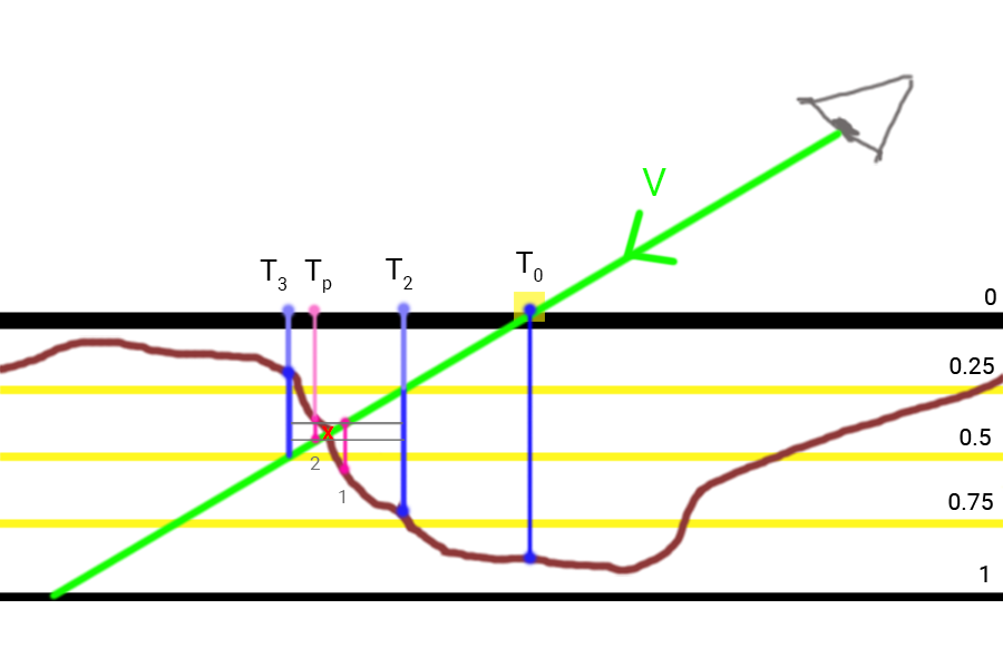
The image shows that after finding the points $$$T_2$ and $$$T_3$ we halve the layer size and the size of the offset of the texture coordinates, which gives us the first iteration point of the binary search (1). Since the sample size in it turned out to be greater than the current depth of the layer, we once again halve the parameters and shift along $$$\ color {green} {\ bar {V}}$ , getting point (2) with texture coordinates $$$T_p$ , which will be the result of Steep PM for two iterations of the binary search.

Shader code:

 //  : inTexCoords -   , // inViewDir -      - //  : lastDepthValue –      //      vec2 reliefPM(vec2 inTexCoords, vec3 inViewDir, out float lastDepthValue) { // ====== // ,   Steep PM // ====== const float _minLayers = 2.; const float _maxLayers = 32.; float _numLayers = mix(_maxLayers, _minLayers, abs(dot(vec3(0., 0., 1.), inViewDir))); float deltaDepth = 1./_numLayers; // uDepthScale –     PM vec2 deltaTexcoord = uDepthScale * inViewDir.xy/(inViewDir.z * _numLayers); vec2 currentTexCoords = inTexCoords; float currentLayerDepth = 0.; float currentDepthValue = depthValue(currentTexCoords); while (currentDepthValue > currentLayerDepth) { currentLayerDepth += deltaDepth; currentTexCoords -= deltaTexcoord; currentDepthValue = depthValue(currentTexCoords); } // ====== //   Relief PM // ====== //         deltaTexcoord *= 0.5; deltaDepth *= 0.5; //      ,   Steep PM currentTexCoords += deltaTexcoord; currentLayerDepth -= deltaDepth; //    … const int _reliefSteps = 5; int currentStep = _reliefSteps; while (currentStep > 0) { currentDepthValue = depthValue(currentTexCoords); deltaTexcoord *= 0.5; deltaDepth *= 0.5; //       , //       if (currentDepthValue > currentLayerDepth) { currentTexCoords -= deltaTexcoord; currentLayerDepth += deltaDepth; } //       else { currentTexCoords += deltaTexcoord; currentLayerDepth -= deltaDepth; } currentStep--; } lastDepthValue = currentDepthValue; return currentTexCoords; } 

There is also a small addition to adding shading from a selected light source to the calculation algorithm. I decided to add it, since technically the calculation method is identical to that discussed above, but the effect is still interesting and adds detail.

Essentially, the same Steep PM is used, but the search goes not deep into the simulated surface along the line of sight, but from the surface, along the vector to the light source$$$\color{green}{\bar{L}}$ .This vector is also transferred to the tangent space and is used to determine the magnitude of the displacement of texture coordinates. At the output of the method, we obtain the real coefficient of illumination in the interval [0, 1], which is used to modulate the diffuse and specular components in the illumination calculations.
To determine the shading with sharp edges, just walk along the vector$$ˉ L until a point lies beneath the surface. As soon as such a point is found, we take the luminance factor of 0. If we reach zero depth without meeting the point lying below the surface, then the luminance factor is 1.To determine shading with soft edges, you need to check several points lying on the vector$\color{green}{\bar{L}}$

$$ˉ L and under the surface. The shading coefficient is taken to be equal to the difference between the depth of the current layer and the depth from the depth map. It also takes into account the removal of the next point from the fragment in question in the form of a weighting factor equal to (1.0 - stepIndex / numberOfSteps). At each step, the partial luminance factor is determined as:$\color{green}{\bar{L}}$

$$

$$PSF_i=(layerHeight_i - heightFromtexture_i)*(1.0-\frac{i}{numSteps})$$

The end result is the maximum coefficient of illumination of all partial:

$$

$$SF=max(PSF_i)$$

Scheme of the method:

The progress of the method for the three iterations in this example:

• Initialize the total light factor to zero.
• Take a step along the vector $$ˉ L , getting to the point$\color{green}{\bar{L}}$$$$H_a$ . The depth of the point is clearly less than the sample from the map. $$H ( T L 1 ) - it is below the surface. Here we made the first check and, keeping in mind the total number of checks, we find and save the first partial light factor: (1.0 - 1.0 / 3.0).$H(T_{L1})$
• Take a step along the vector $$ˉ L , getting to the point$\color{green}{\bar{L}}$$$$H_b$ . The depth of the point is clearly less than the sample from the map. $$H ( T L 2 ) - it is under the surface. The second check and the second partial coefficient: (1.0 - 2.0 / 3.0).$H(T_{L2})$
• We take one more step along the vector and get to the minimum depth of 0. We stop the movement.
• Determination of the result: if no points were found under the surface, then we return a coefficient equal to 1 (no shading). Otherwise, the resulting coefficient becomes the maximum of the calculated partial ones. For use in calculating lighting, we subtract this value from one.

Shader code example:

 //  : inTexCoords -   , // inLightDir -       - //  : inLastDepth –    , //      PM //       //    float getParallaxSelfShadow(vec2 inTexCoords, vec3 inLightDir, float inLastDepth) { float shadowMultiplier = 0.; //      , //    float alignFactor = dot(vec3(0., 0., 1.), inLightDir); if (alignFactor > 0.) { //   :  ,  //  ,     const float _minLayers = 16.; const float _maxLayers = 32.; float _numLayers = mix(_maxLayers, _minLayers, abs(alignFactor)); float _dDepth = inLastDepth/_numLayers; vec2 _dtex = uDepthScale * inLightDir.xy/(inLightDir.z * _numLayers); //  ,    int numSamplesUnderSurface = 0; //       //     L float currentLayerDepth = inLastDepth - _dDepth; vec2 currentTexCoords = inTexCoords + _dtex; float currentDepthValue = depthValue(currentTexCoords); //    float stepIndex = 1.; // ,       … while (currentLayerDepth > 0.) { //     ,     //       if (currentDepthValue < currentLayerDepth) { numSamplesUnderSurface++; float currentShadowMultiplier = (currentLayerDepth - currentDepthValue)*(1. - stepIndex/_numLayers); shadowMultiplier = max(shadowMultiplier, currentShadowMultiplier); } stepIndex++; currentLayerDepth -= _dDepth; currentTexCoords += _dtex; currentDepthValue = depthValue(currentTexCoords); } //      ,   //      1 if (numSamplesUnderSurface < 1) shadowMultiplier = 1.; else shadowMultiplier = 1. - shadowMultiplier; } return shadowMultiplier; } 

The coefficient obtained is used to modulate the result of the work used in the examples of the Blinna-Phong lighting model:

 [...] //      vec3 fullColorADS = ambientTerm + attenuation * (diffuseTerm + specularTerm); //     -  fullColorADS *= pmShadowMultiplier; return fullColorADS; 

Comparison of all methods in one collage, the volume of 3Mb.

Also a video comparison:

Additional materials

• Parallax Occlusion Mapping in GLSL : A great lesson on Parallax Mapping from sunandblackcat.com .
• How Parallax Displacement Mapping Works : A video tutorial explaining well the details of TheBennyBox Parallax Mapping .

PS : We have a telegram-konf to coordinate transfers. If there is a serious desire to help with the translation, then you are welcome!