The general essence of sorting inserts is as follows:
- The elements in the unsorted part of the array are moved.
- Each element is inserted into the sorted part of the array at the place where it should be.
This is, in principle, all you need to know about sorting inserts. That is, sorting inserts always divide the array into 2 parts - sorted and unsorted. Any item is extracted from the unsorted part. Since the other part of the array is sorted, you can quickly find your place for this extracted element in it. The element is inserted where necessary, with the result that the sorted part of the array is increased, and the unsorted part is reduced. Everything. By this principle all sorting inserts work.
The weakest point in this approach is inserting an element into the sorted part of the array. In fact, this is not easy, and what tricks you just have to go to complete this step.
Sort by simple inserts
We pass through the array from left to right and process each element in turn. To the left of the next element, we increase the sorted part of the array, to the right, as the process evaporates, the unsorted one slowly evaporates. In the sorted part of the array, the insertion point is searched for the next element. The element itself is sent to the buffer, with the result that a free cell appears in the array - this allows you to move the elements and release the insertion point.
def insertion(data): for i in range(len(data)): j = i - 1 key = data[i] while data[j] > key and j >= 0: data[j + 1] = data[j] j -= 1 data[j + 1] = key return data
On the example of simple inserts, the main advantage of most (but not all!) Sorts of inserts looks indicative, namely - very fast processing of almost ordered arrays:
In this situation, even the most primitive implementation of sorting inserts is likely to overtake the super-optimized algorithm of some sort of quick sorting, including on large arrays.
This is facilitated by the very basic idea of this class - the transfer of elements from the unsorted part of the array to the sorted one. With close proximity of the largest data, the insertion point is usually close to the edge of the sorted part, which allows insertion with the least overhead.
There is nothing better to handle almost ordered arrays than sorting inserts. When you find information somewhere that the best time complexity of sorting by inserts is
O ( n ) , then most likely it means a situation with almost ordered arrays.
Sort simple inserts with binary search

Since the insertion point is searched for in the sorted part of the array, the idea to use binary search suggests itself. Another thing is that the search for the insertion point is not critical for the time complexity of the algorithm (the main resource eater is the stage of inserting an element into the position found), so this optimization does little here.
In the case of an almost sorted array, binary search may work even slower, since it starts from the middle of the sorted area, which is likely to be too far from the insertion point (and the usual search from the element position to the insertion point will take fewer steps if the data in the array as a whole are ordered).
def insertion_binary(data): for i in range(len(data)): key = data[i] lo, hi = 0, i - 1 while lo < hi: mid = lo + (hi - lo) // 2 if key < data[mid]: hi = mid else: lo = mid + 1 for j in range(i, lo + 1, -1): data[j] = data[j - 1] data[lo] = key return data
In defense of the binary search, I note that he can say the decisive word in the effectiveness of other sorting inserts. Thanks to him, in particular, such algorithms as librarian sorting and solitaire sorting come out on the average time complexity
O ( n log n ) . But about them later.
Pair sorting with simple inserts
Modification of simple inserts, developed in the secret laboratories of the corporation Oracle. This sorting is included in the JDK package and is part of the Dual-Pivot Quicksort. Used for sorting small arrays (up to 47 elements) and sorting small areas of large arrays.

Not one, but two immediately standing elements are sent to the buffer. First, a larger element of the pair is inserted, and immediately after it, the simple insert method is applied to the smaller element of the pair.
What does this give? Savings for handling a smaller item of a pair. For it, the search for the insertion point and the insertion itself are performed only on that sorted part of the array, which does not include the sorted area used to process the larger element of the pair. This becomes possible because the larger and smaller elements are processed immediately one after the other in one pass of the outer loop.
This does not affect the average time complexity (it remains equal to
O ( n 2 )), but pair inserts work a little faster than usual ones.
I illustrate the algorithms in Python, but here I’ll give the source (modified for readability) in Java:
for (int k = left; ++left <= right; k = ++left) {
Shell sort

In this algorithm, there is a very ingenious approach in determining which part of the array is considered to be sorted. In simple inserts, everything is simple: from the current element everything that is on the left is already sorted, everything on the right is not yet sorted. Unlike simple inserts, Shell sorting does not try to form a strictly sorted part of the array immediately to the left of the element. It creates an
almost sorted part of the array to the left of the element and does it fairly quickly.
Sorting Shell shelves the current element in the buffer and compares it with the left side of the array. If it finds more elements on the left, it shifts them to the right, freeing up space for insertion. But at the same time, it takes not the entire left-hand side, but only a certain group of elements from it, where the elements are spaced apart from one another by a certain distance. Such a system allows you to quickly insert elements into approximately the area of the array where they should be.
With each iteration of the main loop, this distance gradually decreases and when it becomes equal to one, the Shell sort at this moment turns into a classical sort with simple inserts, which were given for processing an almost sorted array. A nearly sorted array sorting inserts into fully sorted converts quickly.
def shell(data): inc = len(data) // 2 while inc: for i, el in enumerate(data): while i >= inc and data[i - inc] > el: data[i] = data[i - inc] i -= inc data[i] = el inc = 1 if inc == 2 else int(inc * 5.0 / 11) return data
Sorting the hairbrush in a similar way improves bubble sorting, due to which the time complexity of the algorithm with
O ( n 2 ) jumps right up to
O ( n log n ) . Alas, but Shell fails to repeat this feat - the best time complexity reaches
O ( n log 2 n ) .
A few habstats are written about Shell sorting, so we will not be overloaded with information and move on.
Tree sort
Sorting the tree at the expense of additional memory quickly solves the problem with the addition of the next element in the sorted part of the array. And in the role of the sorted part of the array is a binary tree. The tree is formed literally on the fly when sorting elements.
An element is compared first with the root, and then with more nested nodes according to the principle: if the element is less than a node, then we go down the left branch, if not less, then we go down the right branch. A tree constructed according to this rule can then be easily circumvented so as to move from nodes with smaller values to nodes with large values (and thus get all the elements in ascending order).
The main snag of sorting inserts (the cost of inserting an element in its place in the sorted part of the array) is solved here, the construction is quite operational. In any case, to release the insertion point, it is not necessary to slowly move the caravans of elements as in the previous algorithms. It would seem that here it is, the best of sorting inserts. But there is a problem.
When you get a beautiful symmetric Christmas tree (the so-called ideally balanced tree) as in the animation three paragraphs above, the insertion occurs quickly, because the tree in this case has the lowest possible level of nesting. But a balanced (or at least close to that) structure from a random array is rarely obtained. And the tree, most likely, will be imperfect and unbalanced - with warps, littered horizon and an excess of levels.
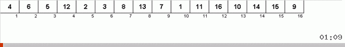
Random array with values from 1 to 10. Elements in this order generate an unbalanced binary tree: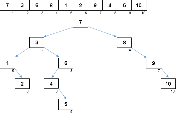
A little tree to build, it still needs to be circumvented. The more imbalance - the stronger the algorithm for traversing the tree will slip. Here, as the stars would say, a random array can generate both an ugly snag (which is more likely) and a tree-like fractal.
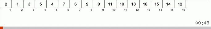
The values of the elements are the same, but the order is different. A balanced binary tree is generated: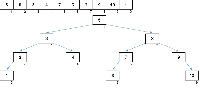
 On a beautiful sakura
Not enough petal:
Binary tree of tens.The problem of unbalanced trees is solved by inversion sorting, which uses a special kind of binary search tree - splay tree. This is a wonderful transforming tree, which after each operation is rebuilt into a balanced state. About this will be a separate article. By that time, I will prepare and implement in Python for both Tree Sort and Splay sort.
Well, we briefly went through the most popular sorting inserts. Simple inserts, Shell and binary tree we all know from school. And now we will consider other representatives of this class, not so widely known.
Wiki / Wiki -
Inserts / Insertion , Shell / Shell , Tree / TreeArticles series:
Who uses AlgoLab - I recommend updating the file. I have added simple binary search and pair inserts to this application. I also completely rewrote the visualization for Shell (in the previous version there was no idea what it was) and added highlighting of the parent branch when inserting an element into a binary tree.