Software implementation of the IIR filter in the information-measuring channel

Information about the state of the environment or, for example, a certain control object can be obtained by measuring the current values ​​of parameters characterizing certain properties of the environment or object. To receive, process and transmit such information by technical means, the value of the measured parameter must be converted by automatic measuring devices into a signal of measuring information. To do this, they implement the information-measuring channel ( IIC ) as a set of technical means, each of which will perform its specific function, ranging from the perception of the measured value to the receipt of measuring information in a form that is convenient for human perception or for further processing. And everything is good, but here along the path of the information to the useful signal y (t) of the measuring information, the interference e (t) is superimposed - a random function of time that can simulate both the random error of the measuring transducer and electrical pickups in the connecting wires and random pulsations measured parameter, and other factors.

On this basis, there arises the problem of primary information processing in the SEC - filtering the signal y (t) of the measurement information from random interference e (t). In general, filtering methods are based on the difference in the frequency spectra of the functions y (t) and e (t), and the interference is considered to be more high-frequency.

Synthesis of the optimal implemented filter is a difficult task, which requires the precise specification of the characteristics of the useful signal and interference. Therefore, in practice, the transfer function of the filter is usually specified and limited to parametric synthesis using simple filtering algorithms.

Filtering methods are carried out both at the software level and at the hardware level. For example, in the BMP280 sensor (BOSCH) it is possible to connect an IIR filter at the hardware level, changing the filter coefficient k, [1], as necessary.

IIR filter

Filters with infinite impulse response refer to recursive filters and calculate the output signal based on the values ​​of the previous input and output samples. Theoretically, the impulse response of an IIR filter never reaches zero, so the output is infinite in duration.

In general, the filtering algorithm for a one-dimensional scalar digital filter is written as [2]:

$$$y [n] = T (x [n], x [n-1], ..., x [n-M], y [n-1], ..., y [n-N], n)$, (one),
where T is a scalar function of one variable.

The function T depends on the current input signal x [n], and previous: M samples of the input signal and N samples of the output signal

The output of the IIR filter is described by a difference equation of the form:

(2)
where x [n], y [n] is the input and output of the filter, respectively, { $$${a_k}$} - a set of direct coefficients, M - the number of direct coefficients, { $$${b_k}$} Is the set of inverse coefficients, N is the number of inverse coefficients.

Applying a z-transform to both sides of equation (2), we get:

(3).

Then the transfer function of the filter will look like this:

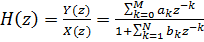
(four)

Algorithm for filtering one-dimensional IIR filter

In general, the filtering algorithm for a one-dimensional scalar stationary recursive filter looks like this:

$$$y [n] = T (x [n], y [n-1])$. (five)

We now write the difference equation for the IIR filter in the form [1]:

(6),
where k is the filter coefficient;
or
$$$y [n] = ay [n-1] + bx [n]$(7),
Where - inverse and direct filter coefficients, respectively.

From (7) it is obvious that when k = 1, the output signal of the filter will repeat the input signal, and as the filter coefficient k increases, the weight of the previous filtered signal goes to 1, and the weight of the measured value goes to 0.

Algorithm (6) is implemented using the example of an absolute atmospheric pressure information channel for the BMP280 sensor, at the software level in the Arduino Software development environment (IDE), Listing 1. The electrical circuitry of the IIC components connections is shown in Fig. 1. A general view of the prototype of the IIC of absolute atmospheric pressure is presented in Fig. 2. The prototype provides the ability to change the filtration coefficient in the range of 1 ... 50 in increments of 1, by rotating the potentiometer knob. On the sign LCD screen, the measured pressure value is displayed (with k = 1) or the filtered value (with k = 2 ... 50), and the value of the filter coefficient k.



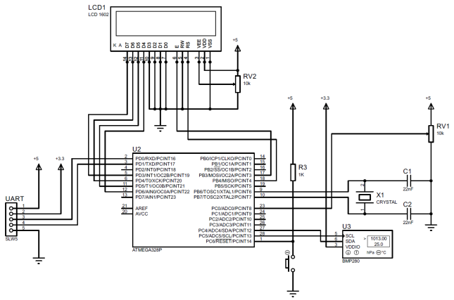Fig. 1 - Electrical wiring diagram of the components of the prototype IIC


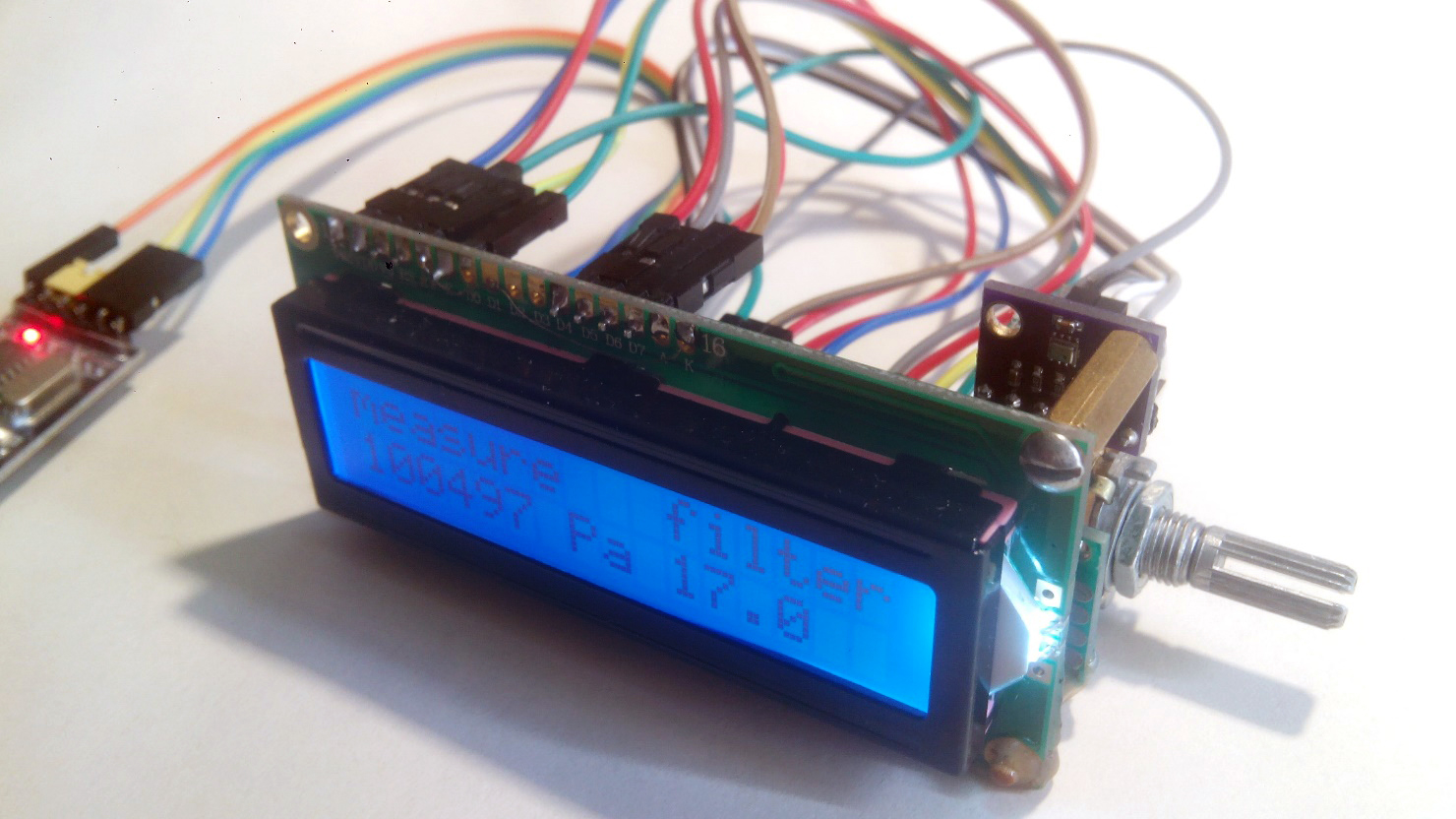Fig. 2 - General view of the prototype of the IIC

Python script for IIR filter research

Listing 2 shows a Python script for examining IIR filters. The filter coefficient k is prescribed in the script. The measured pressure values ​​are sequentially read from the virtual COM port and filtered. The graphical window and the console display the measured and filtered values ​​of the measured parameter in real time. The results of the experiment are recorded by the table in a file, and time graphs of the measured and filtered values ​​are displayed in the graphic window.

Experimental results

   : 33    : 6  : COM6 : n -  ; P - , ;     n P 0 100490.00 100490.00 1 100488.00 100489.71 2 100487.00 100489.33 3 100488.00 100489.14 4 100488.00 100488.97 … 30 100486.00 100488.14 31 100492.00 100488.70 32 100489.00 100488.74   : 16.028, c   : 0.500875, c     275_count.txt  Ctrl-C,   

findings

The filtering algorithm is very simple in software implementation and, in practice, can be used in the IIC, similar to that considered in this article.
The work was attended by Losikhin DA, s.v. kaf KITiM .

Information sources

1. BMP280 Digital Pressure Sensor
   
2. Infinite impulse response filter