iMaterialist Furniture Challenge or 50 shades of chairs

Recently, Kaggle ended the iMaterialist Challenge (Furniture) competition, the task of which was to classify images into 128 types of furniture and household items (the so-called fine-grained classification, where classes are very close to each other).

In this article I will describe the approach that third place brought to us from m0rtido , but before getting to the point, I suggest using the natural neural network in my head to solve this problem and divide the chairs in the photo below into three classes.




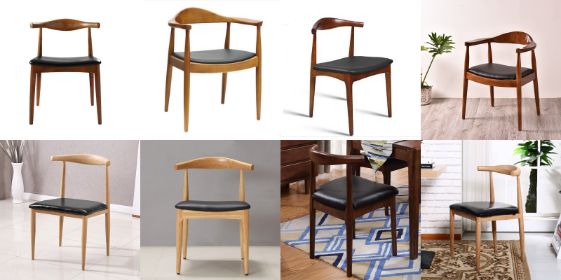
You guessed? Me neither.

But stop, first things first.

Formulation of the problem

In the competition, we were given a data set in which 128 classes of ordinary household objects were represented, such as chairs, televisions, pans and pillows in the form of anime characters.
The training part of the dataset consisted of ~ 190 thousand images (the exact number is difficult, because the participants were given only a set of URLs for download, some of which, of course, did not work), and the distribution of classes was far from uniform (see clickable image below) .



The test dataset was presented with 12800 pictures, and it was perfectly balanced: there were 100 images for each class. A validation dataset was also issued, which also had a balanced distribution of classes and was exactly half the size of the test.

Task evaluation metric was $$$error \ _rate = 1 - accuracy$.

How did we decide?

First of all, we downloaded the data and looked through a small part with our eyes. Instead of many images, a 1x1 image or a placeholder with an error was downloaded. We immediately deleted such images with a script.

Transfer learning

It was obvious that with the available number of images and time limits, it’s not very sensible to train neural networks from scratch on this dataset. Instead, we used the transfer learning approach, the idea of ​​which is this: the weights of a network trained on one task can be used for a completely different data set and get a decent quality, or even an increase in accuracy compared to learning from scratch.

How does it work? Hidden layers in deep neural networks act as feature extractors, extracting features that are then used by the upper layers directly for classification.

We took advantage of this by training a number of deep CNNs previously trained on ImageNet. For these purposes, we used Keras and its model zoo, where there was enough code like this for loading the finished architecture:

base_model = densenet.DenseNet201(weights='imagenet', include_top=False, input_shape=(img_width, img_height, 3), pooling='avg') 

After that, we extracted the so-called bottleneck-signs (features at the exit from the last convolutional layer) from the network and trained softmax with dropout on top of them.

Then, we trained the “top” weights with the convolutional part of the network and trained the entire network at once.


With a similar fine-tuning of networks, we managed to try the following hacks:

1. Data augmentation . To combat overfitting, we used very hard augmentation: horizontal reflection, zoom, pan, tilt, tilt, add color noise, color channel shifts, training at five points (angles and center of the image). We also wanted to try FancyPCA , but could not because of the lack of computing resources.
2. Tta . To predict classes on validation and test, we used augmentation, a little less aggressive than during training, and averaged the results of predictions to increase accuracy.
3. Cyclic Learning rate . Cyclic increase and decrease in the rate of training helped the models not to get stuck in local minima.
4. Training models on a subset of classes . As it can be understood from the picture above the cut, in the dataset there were very close classes to each other. So close that on certain clusters of objects (for example, on chairs and armchairs, which were already represented by 8 classes), our models were mistaken much more than on other types of objects. We tried to train a separate CNN to recognize only chairs, hoping that such a network would learn to distinguish between different types of chairs better than a general-purpose network, but this approach did not give an increase in accuracy.
   
   Why? Partially the answer to this question is presented in the picture before the cat - the classes were so similar that even with the initial markup of the data, the people who stamped the classes could not distinguish between them, therefore, it would still not be possible to squeeze good accuracy from these data.
5. Spatial Transformer Network . Despite the fact that we trained one of the networks with her and got pretty good accuracy, unfortunately she did not enter the final submit.
6. Weighted loss function . To compensate for the unbalanced distribution of classes, we used weighted loss. This helped both in learning softmax- "tops", and with further training of the whole network. Weights were calculated using the function from scikit-learn and then passed to the model's fit method:

 train_labels = utils.to_categorical(train_generator.classes) y_integers = np.argmax(train_labels, axis=1) class_weights = compute_class_weight('balanced', np.unique(y_integers), y_integers) 

Networks trained in this way accounted for 90% of our final ensemble.

Bottleneck Stacking

Disclaimer: never repeat the technique described later in real life.

So, as we decided in the previous section, bottleneck features from networks trained on ImageNet can be used for classification in other tasks. m0rtido decided to go further, and proposed the following strategy:

1. Let's take all the pre-trained architectures available to us (in particular, NasNet Large, InceptionV4, Vgg19, Vgg16, InceptionV3, InceptionResnetV2, Resnet-50, Resnet-101, Resnet-152, Xception, Densenet-169, Densenet-121, Densenet-201 were taken ) and extract bottleneck signs from them. We also calculate the signs for the reflected variants of the pictures (such a minimalistic augmentation).
2. We will reduce the dimensionality of the signs of each of the models three times with the help of PCA, so that they fit normally in the 16 Gb RAM available to us.
3. We concatenate these signs into one large feature vector.
4. Let's train on top of all this one multilayer perceptron and generate predictions. Also we will teach with splitting into folds and average all these predictions.

The resulting monstrous stacking gave a huge increase in accuracy to the overall ensemble.

Model Ensemble

After all of the above, we had about two dozen extinguished convolution networks, as well as two perceptrons on top of the bottleneck signs. There was a question: how to get a single prediction from this?

In an amicable way, in the best traditions of Kaggle, we had to do stacking on top of all this, but in order to do OOF stacking, we had neither time nor GPU, and learning a top-level model on validation hold led to a very large overfit. Therefore, we decided to implement a fairly simple algorithm for the greedy creation of an ensemble:

1. Initialize an empty ensemble.
2. We try to add each model in turn and count the score. Choose the model that raises the metric the most and add it to the ensemble. The results of the prediction models in the ensemble are simply averaged.
3. If none of the models improves the performance, go through the ensemble and try to remove models from it. If you manage to remove some model so that the score improves, do it and go back to step 2.

As a metric was selected $$$score = 0.5 * accuracy - logloss$. This formula was chosen empirically so that $$$accuracy$and $$$logloss$obtained approximately the same scale. Such an integral metric correlated well with $$$accuracy$both on validation and on a public leaderboard.

In addition, the fact that at each iteration we added or removed one model (that is, the model weights always remained integers) played the role of a sort of regularization, not allowing the ensemble to overfill under the validation data set.

As a result, the following models entered the ensemble:

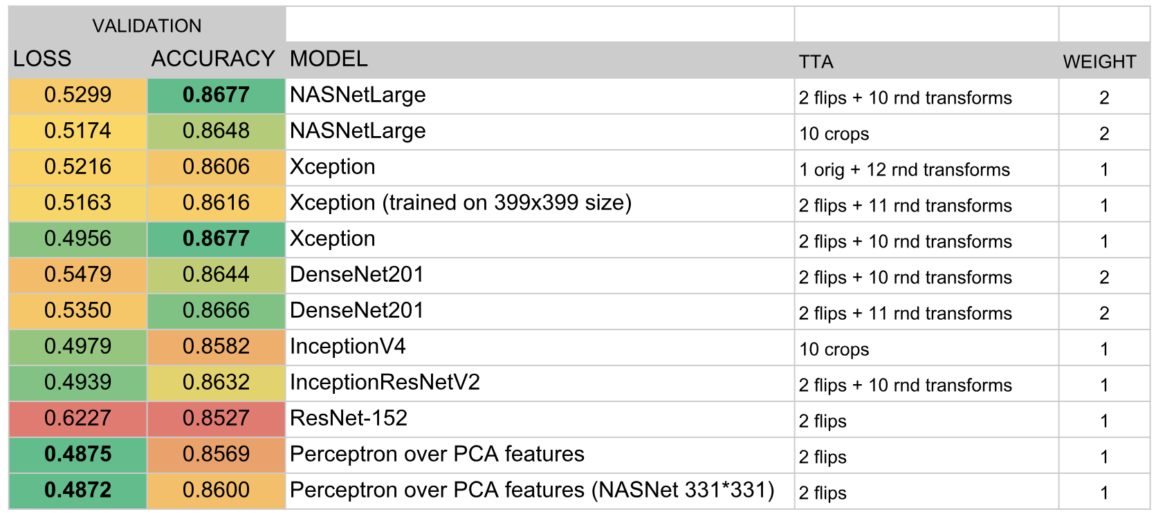
results

According to the results of the competition, we took the third place. The key to success was, I think, the good choice of the ensemble algorithm and the huge amount of time that m0rtido and I invested in learning a large number of models.