If we describe in a couple of sentences on what basis do sorting exchanges work, then:

1. The array elements are compared in pairs
2. If the element on the left is ^* more than the element on the right, then the elements are swapped.
3. Repeat steps 1-2 until the array is sorted.

^{* - the element on the left is the element from the compared pair, which is closer to the left edge of the array. Accordingly, the element on the right is closer to the right edge.}

Immediately I apologize for repeating the well-known material, it is unlikely that even one of the algorithms in the article will be a revelation to you. About these sortings on Habré was written repeatedly (including me - 1 , 2 , 3 ) and it is asked, why again to return to this topic? But since I decided to write a coherent series of articles about all sorts in the world , I have to at least take a quick look at exchange methods. When considering the following classes, there will already be many new (and little-known) algorithms that deserve some interesting articles.

Traditionally, “exchangers” include sorting, in which elements change (pseudo) randomly (bogosort, bozosort, permsort, etc.). However, I did not include them in this class, as there are no comparisons. There will be a separate article about these sortings, where we will have plenty to philosophize about the theory of probability, combinatorics and the thermal death of the Universe.

Silly sort :: Stooge sort

1. We compare (and, if necessary, change) the elements at the ends of the subarray.
2. We take two thirds of the subarray from its beginning and recursively apply a common algorithm to these 2/3.
3. We take two thirds of the subarray from its end and recursively apply the general algorithm to these 2/3.
4. And again we take two thirds of the subarray from its beginning and to these 2/3 we recursively apply a common algorithm.

Initially, the subarray is the entire array. And then the recursion splits the parent subarray by 2/3, makes comparisons / exchanges at the ends of the crushed segments and eventually arranges everything.

def stooge_rec(data, i = 0, j = None): if j is None: j = len(data) - 1 if data[j] < data[i]: data[i], data[j] = data[j], data[i] if j - i > 1: t = (j - i + 1) // 3 stooge_rec(data, i, j - t) stooge_rec(data, i + t, j) stooge_rec(data, i, j - t) return data def stooge(data): return stooge_rec(data, 0, len(data) - 1) 

It looks schizophrenic, but nevertheless it is 100% correct.

Sluggish sort :: Slow sort

And here we see recursive mysticism:

1. If the subarray consists of a single element, then we complete the recursion.
2. If a subarray consists of two or more elements, then divide it in half.
3. We apply a recursive algorithm to the left half.
4. We apply the recursive algorithm to the right half.
5. Elements at the ends of the subarray are compared (and changed if necessary).
6. Recursively apply the algorithm to a subarray without the last element.

Initially, a subarray is the entire array. And the recursion will continue to halve, compare and change until everything sorts.

 def slow_rec(data, i, j): if i >= j: return data m = (i + j) // 2 slow_rec(data, i, m) slow_rec(data, m + 1, j) if data[m] > data[j]: data[m], data[j] = data[j], data[m] slow_rec(data, i, j - 1) def slow(data): return slow_rec(data, 0, len(data) - 1) 

It looks like nonsense, but the array is ordered.

Why do StoogeSort and SlowSort work correctly?

An inquisitive reader will ask a reasonable question: why do these two algorithms work at all? They seem to be simple, and not particularly obvious that something can be sorted.

Let's first analyze the Slow sort. The last point of this algorithm hints that the recursive efforts of sluggish sorting are aimed only at putting the largest element in the subarray in the rightmost position. This is especially noticeable if the algorithm is applied to a back-ordered array:



It is clearly seen that at all levels of recursion, the maxima quickly migrate to the right. Then these maxima, which turned out to be where they are needed, are turned off from the game: the algorithm calls itself — but without the last element.

Similar magic happens in Stooge sort:



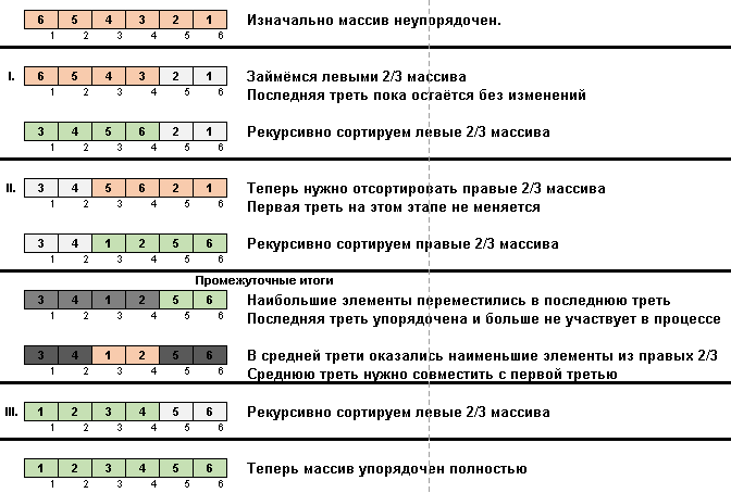
In fact, there is also an emphasis on maximum elements. Only Slow sort moves them to the end one by one, and the Stooge sort third of the subarray elements (the largest of them) moves to the right third of the cell space.

We proceed to the algorithms, where everything is already quite obvious.

Dull sort :: Stupid sort

Very careful sorting. It goes from the beginning of the array to the end and compares the neighboring elements. If two neighboring elements had to be swapped, then sorting just in case returns to the very beginning of the array and starts all over again.

 def stupid(data): i, size = 1, len(data) while i < size: if data[i - 1] > data[i]: data[i - 1], data[i] = data[i], data[i - 1] i = 1 else: i += 1 return data 

Dwarf sort :: Gnome sort

Almost the same thing, but here the exchange sorting does not return to the very beginning of the array, but takes only one step back. This, it turns out, is quite enough to sort everything out.

 def gnome(data): i, size = 1, len(data) while i < size: if data[i - 1] <= data[i]: i += 1 else: data[i - 1], data[i] = data[i], data[i - 1] if i > 1: i -= 1 return data 

Optimized gnome sorting

But you can save not only on the retreat, but also when moving forward. With several exchanges in a row, you have to take as many steps back. And then you have to go back (comparing along the way elements that are already ordered relative to each other). If you memorize the position from which the exchanges began, then you can immediately jump to this position when the exchanges are completed.

 def gnome(data): i, j, size = 1, 2, len(data) while i < size: if data[i - 1] <= data[i]: i, j = j, j + 1 else: data[i - 1], data[i] = data[i], data[i - 1] i -= 1 if i == 0: i, j = j, j + 1 return data 

Bubble sort :: Bubble sort

In contrast to the stupid and dwarf sorting, there are no returns during the exchange of items in the bubbly - it continues to move forward. Having reached the end, the largest element of the array is moved to the very end.

Then sorting repeats the whole process anew, with the result that the second element in order of seniority is in the penultimate place. At the next iteration, the third largest element is the third from the end, and so on.

 def bubble(data): changed = True while changed: changed = False for i in range(len(data) - 1): if data[i] > data[i+1]: data[i], data[i+1] = data[i+1], data[i] changed = True return data 

Optimized bubble sorting

You can gain a little on the aisles at the beginning of the array. In the process, the first elements are temporarily ordered relative to each other (this sorted part is constantly changing in size - then decreases, then increases). This is easily fixed and with a new iteration you can simply jump over a group of such elements.
_{(I’ll add a proven implementation on Python a little later. I didn’t have time to prepare it.)}

Shaker sort :: Shaker sort
(Cocktail Sort :: Cocktail sort)

A kind of bubble. On the first pass, as usual - push the maximum to the end. Then abruptly turn around and push at least to the beginning. The sorted extreme areas of the array increase in size after each iteration.

 def shaker(data): up = range(len(data) - 1) while True: for indices in (up, reversed(up)): swapped = False for i in indices: if data[i] > data[i+1]: data[i], data[i+1] = data[i+1], data[i] swapped = True if not swapped: return data 

Even-odd sort :: Odd-even sort

Again, iteration over pairwise comparison of neighboring elements when moving from left to right. Only first we compare pairs in which the first element is odd in a row, and the second is even (that is, the first and second, third and fourth, fifth and sixth, etc.). And then vice versa - even + odd (second and third, fourth and fifth, sixth and seventh, etc.). In this case, many large elements of the array at one iteration at the same time make one step forward (the largest bubble in the iteration reaches the end, but the remaining rather big ones all remain in place).

By the way, this was originally a parallel sort with complexity O (n). It will be necessary in AlgoLab to implement in the section "Parallel sorting".

 def odd_even(data): n = len(data) isSorted = 0 while isSorted == 0: isSorted = 1 temp = 0 for i in range(1, n - 1, 2): if data[i] > data[i + 1]: data[i], data[i + 1] = data[i + 1], data[i] isSorted = 0 for i in range(0, n - 1, 2): if data[i] > data[i + 1]: data[i], data[i + 1] = data[i + 1], data[i] isSorted = 0 return data 

Comb sorting :: Comb sort

The most successful modification of the bubble. The algorithm competes in speed with quick sorting.

In all previous variations we compared the neighbors. And here, first considered are pairs of elements that are at a maximum distance from each other. With each new iteration, this distance is evenly narrowed.

 def comb(data): gap = len(data) swaps = True while gap > 1 or swaps: gap = max(1, int(gap / 1.25)) # minimum gap is 1 swaps = False for i in range(len(data) - gap): j = i + gap if data[i] > data[j]: data[i], data[j] = data[j], data[i] swaps = True return data 

Quick sort :: Quick sort

Well, the most advanced exchange algorithm.

1. Divide the array in half. The middle element is the reference.
2. Moving from the left edge of the array to the right, until we find an element that is larger than the reference.
3. We move from the right edge of the array to the left, until we find an element that is smaller than the reference.
4. Swap the two elements found in points 2 and 3.
5. We continue to perform paragraphs 2-3-4 until a meeting occurs as a result of mutual movement.
6. At the meeting point, the array is divided into two parts. We recursively apply the quick sort algorithm to each part.

Why does this work? To the left of the meeting point are elements that are smaller or equal than the reference. To the right of the meeting point are elements larger or equal than the reference. That is, any element from the left side is less than or equal to any element from the right side. Therefore, at the meeting point, the array can be safely divided into two subarrays and similarly recursively sort each subarray.

 def quick(data): less = [] pivotList = [] more = [] if len(data) <= 1: return data else: pivot = data[0] for i in data: if i < pivot: less.append(i) elif i > pivot: more.append(i) else: pivotList.append(i) less = quick(less) more = quick(more) return less + pivotList + more 

K-sort :: K-sort

On Habré published a translation of one of the articles, which reported on the modification of QuickSort, which is 7 million elements ahead of the pyramidal sorting. By the way, this in itself is a dubious achievement, because the classical pyramidal sorting does not beat performance records. In particular, its asymptotic complexity under no circumstances reaches O (n) (a feature of this algorithm).

But the thing is different. According to the author’s (and, obviously, incorrect) pseudo-code, one doesn’t understand what the main idea of ​​the algorithm is. Personally, I got the impression that the authors are some rogues who acted according to this method:

1. Declare the invention of the super-sorting algorithm.
2. We support the statement with a non-working and incomprehensible pseudocode (like, clever and so clear, and fools are still not understood).
3. We provide graphs and tabs that supposedly demonstrate the practical speed of the algorithm on big data. Due to the absence of a really working code, no one will be able to verify or deny these statistical calculations.
4. We publish nonsense on Arxiv.org under the guise of a scientific article.
5. PROFIT !!!

Perhaps I in vain slander on people and in fact the algorithm is working? Can anyone explain how k-sort works?

UPD. My blatant accusations of the authors of sorting for fraud were untenable :) The user jetsys figured out the pseudocode of the algorithm, wrote a working version in PHP and sent it to me in personal messages:

Announcement

It was all theory, it's time to move on to practice. The next article is testing sorting exchanges on different data sets. We will find out:

• What is the worst sort - silly, sluggish or stupid?
• Do optimization and modification of bubble sorting help greatly?
• Under what conditions do slow algorithms easily get by the speed of QuickSort?

And when we find out the answers to these crucial questions, we can begin to study the next class — sorts by inserts.

Links

Excel-AlgoLab application , with which you can step by step to view the visualization of these (and not only these) sorts.

Wiki / Wiki - Silly / Stooge , Slow , Gnome / Gnome , Bubble / Bubble , Shaker / Shaker , Odd-Even / Odd-Even , Comb / Fast, Quick

Series articles

• Excel application AlgoLab.xlsm
• Exchange sorting
  • Comparing sorting exchanges
• Sorting inserts
• Sort by selection
• Merge sort