In this article we will discuss some algorithms for searching and describing the singular points of images. Here this topic has already been raised , and more than once . I will assume that the basic definitions are already familiar to the reader, consider in detail the heuristic algorithms FAST, FAST-9, FAST-ER, BRIEF, rBRIEF, ORB, and discuss the sparkling ideas underlying them. In part, this will be a free translation of the essence of several articles [1,2,3,4,5], there will be some code for “try”.

FAST algorithm

FAST, first proposed in 2005 in [1], was one of the first heuristic methods to search for singular points, which gained great popularity because of its computational efficiency. To make a decision on whether to consider a given point C special or not, this method considers the brightness of pixels on a circle with a center at point C and a radius of 3:



Comparing the brightness of the pixels of a circle with the brightness of the center C, we obtain for each three possible outcomes (lighter, darker, it seems):

$$$ inline $ \ begin {array} {l} {I_p}> {I_C} + t \\ {I_p} <{I_C} -t \\ {I_C} -t <{I_p} <{I_C} + t \ end {array} $ inline $

Here I is the brightness of the pixels, t is some pre-fixed threshold in brightness.
A point is marked as special if there are n = 12 pixels in a circle that are darker, or 12 pixels that are lighter than the center.

As practice has shown, on average, to make a decision, it was necessary to check about 9 points. In order to speed up the process, the authors first proposed to check only four pixels numbered: 1, 5, 9, 13. If among them there are 3 pixels lighter or darker, then a full check is performed on 16 points, otherwise the point is immediately marked as “ not special. " This greatly reduces the work time, on average it’s enough to make a decision to interview only about 4 points of a circle.

A bit of naive code is here.
Variable parameters (described in the code): the radius of the circle (takes values ​​1,2,3), the parameter n (in the original n = 12), the parameter t. The code opens the file in.bmp, processes the image, saves it to out.bmp. Pictures are ordinary 24-bit.

Build a decision tree, Tree FAST, FAST-9

In 2006, in [2], it was possible to develop an original idea using machine learning and decision trees.

The original FAST has the following disadvantages:

• Several adjacent pixels can be marked as special points. Need some measure of "strength" features. One of the first proposed measures is the maximum value of t, at which the point is still taken as special.
• The fast 4-point test is not generalized for n less than 12. For example, the visually best results of the method are achieved with n = 9, not 12.
• I would like to speed up the algorithm!

Instead of using a cascade of two tests of 4 and 16 points, it is proposed to do everything in one pass through the decision tree. Similarly, the original method will compare the brightness of the center point with the points on the circle, but in such a way as to make a decision as quickly as possible. And it turns out that you can make a decision in just ~ 2 (!!!) comparisons on average.

The most important thing is how to find the right order for comparing points. Find with machine learning. Suppose someone noted for us in the picture many special points. We will use them as a set of teaching examples and the idea is to greedily choose the one that will give the greatest amount of information in this step as the next point. For example, suppose that initially in our sample there were 5 singular points and 5 non-singular points. In the form of a tablet like this:



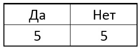
Now we choose one of the pixels p of the circle and for all the special points we will compare the central pixel with the selected one. Depending on the brightness of the selected pixel near each singular point, the table may have the following result:



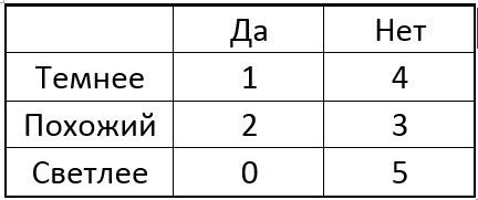
The idea is to choose a point p such that the numbers in the columns of the table are as different as possible. And if now for the new unknown point we get the result of the comparison “Lighter”, then we can immediately say that the point is “not special” (see table). The process continues recursively until the points of only one of the classes fall into each group after dividing it into “darker-like-lighter”. It turns out a tree of the following form:



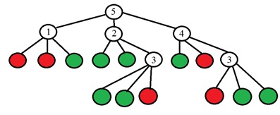
There is a binary value in the leaves of the tree (red is special, green is not special), and in the other vertices of the tree there is the number of the point to be analyzed. More specifically, the original article proposes making the choice of the number of a point for the change in entropy. The entropy of a set of points is calculated:

$$$$ display $$ H = \ left ({c + \ overline c} \ right) {\ log _2} \ left ({c + \ overline c} \ right) - c {\ log _2} c - \ overline c {\ log _2} \ overline c $$ display $$

c is the number of singular points$$ $ inline $ {\ bar c} $ inline $ - the number of non-singular points of the set

Entropy change after processing point p:

$$$$ display $$ \ Delta H = H - {H_ {dark}} - {H_ {equal}} - {H_ {bright}} $$ display $$

Accordingly, a point is selected for which the change in entropy will be maximal. The partitioning process stops when entropy is zero, which means that all points are special, or vice versa - all are not special. With software implementation, after all this, the found decision tree is converted into a set of “if-else” constructions.

The last stage of the algorithm is the operation of suppressing non-maxima in order to get one from several adjacent points. The developers propose using the original measure based on the sum of the absolute differences between the center point and the circle points in this form:

$$$$ display $$ V = \ max \ left ({\ sum \ limits_ {x \ in {S_ {bright}}} {\ left | {{I_x} - {I_p}} \ right | - t, \ sum \ limits_ {x \ in {S_ {dark}}} {\ left | {{I_p} - {I_x}} \ right | - t}}} \ right) $$ display $$

Here$$ $ inline $ {S_ {bright}} $ inline $ and$$ $ inline $ {S_ {dark}} $ inline $ respectively, the pixel groups are lighter and darker, t is the threshold brightness value,$$ $ inline $ {I_p} $ inline $ - the brightness of the central pixel$$ $ inline $ {{I_x}} $ inline $ - the brightness of the pixel on the circle. You can try the algorithm with the following code . The code is taken from OpenCV and freed from all dependencies, just run.

We optimize the decision tree - FAST-ER

FAST-ER [3] is an algorithm of the same authors as the previous one, a fast detector is similarly constructed, an optimal sequence of points is also searched for comparison, a decision tree is also constructed, but by another method - by optimization.

We already understand that the detector can be represented as a decision tree. If we had any criterion for comparing the performance of different trees, then we can maximize this criterion by going through different versions of the trees. And now it is proposed to use “Repeatability” as such a criterion.

Repeatability indicates how well the particular points of the scene are detected from different angles. For a pair of pictures, a dot is called “useful” if it is found on one frame and theoretically can be found on another, i.e. not obstructed by elements of the scene. And a dot is called “repeated” (repeated) if it is found on the second frame, too. Since the optics of the camera is not ideal, the point on the second frame may not be located in the calculated pixel, but somewhere near it. The developers took a neighborhood of 5 pixels. We define recurrence as the ratio of the number of repeated points to the number of useful ones:

$$$$ display $$ R = \ frac {{{N_ {repeated}}}} {{{N_ {useful}}}} $$ display $$

To search for the best detector, an annealing simulation method is used. On Habré there is already a wonderful article about him. Briefly, the essence of the method is as follows:

• Some initial solution of the problem is chosen (in our case it is some kind of detector tree).
• Repeatability is considered.
• The tree is randomly modified.
• If the modified version is better by the repeatability criterion, then the modification is accepted, and if it is worse, it can either be accepted or not, with a certain probability, which depends on a real number called “temperature”. With an increase in the number of iterations, the temperature drops to zero.

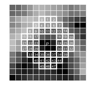
In addition, now not 16 points of a circle, as before, but 47, are involved in the construction of the detector, but the meaning does not change at all:



According to the method of simulating annealing, we define three functions:

• Cost function k. In our case, we use repeatability as the cost. But there is one problem. Imagine that all points on each of the two images are detected as special. Then it turns out that repeatability is 100% is absurd. On the other hand, suppose we have found one singular point in two pictures, and these points coincided - the repeatability is also 100%, but this also does not interest us. Therefore, the authors suggested using the following as a quality criterion:

$$$$ display $$ k = \ left ({1 + {{\ left ({\ frac {{{w_r}}} {R}} \ right)} ^ 2}} \ right) \ left ({1 + \ frac {1} {N} \ sum \ limits_ {i = 1} {{{\ left ({\ frac {{{d_i}}} {{{w_n}}}} \ right)} ^ 2}}} right) \ left ({1 + {{\ left ({\ frac {s} {{{w_s}}}} \ right)} ^ 2}} \ right) $$ display $$

r - repeatability$$ $ inline $ {{d_i}} $ inline $ - the number of detected angles on the frame i, N - the number of frames and s - the size of the tree (the number of vertices). W - custom method parameters.]

• The function of temperature change with time:

$$$$ display $$ T \ left (I \ right) = \ beta \ exp \ left ({- \ frac {{\ alpha I}} {{{I _ {\ max}}}}} \ right) $$ display $$

Where$$ $ inline $ \ alpha, \ beta $ inline $ - coefficients, Imax - the number of iterations.

• The function that generates a new solution. The algorithm makes random tree modifications. First, some vertex is selected. If the selected vertex is a leaf of the tree, then with equal probability we do the following:

1. Replace the vertex with a random subtree of depth 1
2. Change the class of this sheet (singular-smooth point)

If this is NOT a sheet:

1. Replace the number of the tested point with a random number from 0 to 47
2. Replace vertex with random class sheet
3. Swap two subtrees from this vertex

The probability P of making a change at iteration I is:
$$$ inline $ P = \ exp \ left ({\ frac {{k \ left ({i - 1} \ right) - k \ left (i \ right)}} {T}} \ right) $ inline $
k is the cost function, T is the temperature, i is the iteration number.

These modifications to the tree allow both the growth of the tree and its reduction. The method is random, it does not guarantee that you will get the best tree. Run the method many times, choosing the best solution. In the original article, for example, run 100 times per 100,000 iterations each, which takes 200 hours of processor time. As the results show, the result is better than Tree FAST, especially in the noisy pictures.

BRIEF Descriptor

After the singular points are found, their descriptors are calculated, i.e. feature sets characterizing the neighborhood of each singular point. BRIEF [4] is a fast heuristic descriptor built from 256 binary comparisons between pixel brightness in a blurred image. The binary test between points x and y is determined as follows:

$$$$ display $$ \ tau \ left ({P, x, y} \ right): = \ left \ {{\ begin {array} {* {20} {c}} {1: p \ left (x \ right) <p \ left (y \ right)} \\ {0: p \ left (x \ right) \ ge p \ left (y \ right)} \ end {array}} \ right. $$ display $$

The original article examined several ways to select points for binary comparisons. As it turned out, one of the best ways is to select points randomly by a Gaussian distribution around the center pixel. This random sequence of points is selected once and does not change in the future. The size of the considered neighborhood of the point is 31x31 pixels, and the blur aperture is 5.

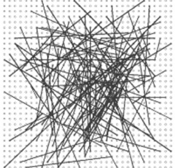
The resulting binary descriptor is resistant to light changes, perspective distortion, quickly calculated and compared, but very unstable to rotation in the image plane.

ORB - fast and efficient

The development of all these ideas was the ORB (Oriented FAST and Rotated BRIEF) algorithm [5], in which an attempt was made to improve the BRIEF performance by rotating the image. It is proposed to first calculate the orientation of the singular point and then carry out binary comparisons already in accordance with this orientation. The algorithm works as follows:

1) Special points are detected using fast tree-like FAST on the original image and on several images from the pyramid of thumbnails.

2) For the detected points, the Harris measure is calculated, candidates with a low Harris measure value are discarded.

3) Calculates the angle of orientation of the singular point. To do this, first calculate the brightness moments for the neighborhood of the singular point:

$$$ inline $ {m_ {pq}} = \ sum \ limits_ {x, y} {{x ^ p} {y ^ q} I \ left ({x, y} \ right)} $ inline $
x, y - pixel coordinates, I - brightness. And then the orientation angle of the feature point:
$$$ inline $ \ theta = {\ rm {atan2}} \ left ({{m_ {01}}, {m_ {10}}} \ right) $ inline $

All this, the authors called the "centroid orientation." As a result, we obtain some direction for the neighborhood of the singular point.

4) Having the orientation angle of a singular point, the sequence of points for binary comparisons in the BRIEF descriptor is rotated in accordance with this angle, for example:



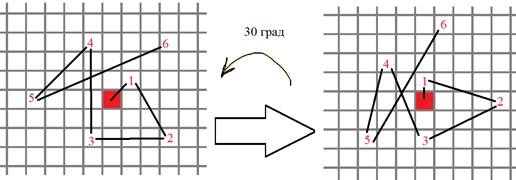
If more formally, new positions for points of binary tests are calculated as follows:

$$$$ display $$ \ left ({\ begin {array} {* {20} {c}} {{x_i} '} \\ {{y_i}'} \ end {array}} \ right) = R \ left (\ theta \ right) \ cdot \ left ({\ begin {array} {* {20} {c}} {{x_i}} \\ {{y_i}} \ end {array}} \ right) $$ display $$

5) A binary descriptor BRIEF is computed from the obtained points.

And on this ... not everything! There is another interesting detail in the ORB that requires separate explanations. The fact is that at the moment when we “turn” all singular points to the zero angle, the random selection of binary comparisons in the descriptor ceases to be random. This leads to the fact that, firstly, some binary comparisons are dependent on each other, secondly, their average is no longer equal to 0.5 (1 - lighter, 0 - darker, when the choice was random, it was on average 0.5) and All this significantly reduces the ability of the descriptor to distinguish particular points from each other.

The solution - you need to choose the "correct" binary tests in the learning process, this idea breathes the same flavor as learning the tree for the FAST-9 algorithm. Suppose we have a bunch of singular points already found. Consider all possible options for binary tests. If the neighborhood is 31 x 31, and the binary test is a pair of 5 x 5 subsets (due to blurring), then there are a lot of choices N = (31-5) ^ 2. The algorithm for finding "good" tests is:

1. We calculate the result of all tests for all special points.
2. Sort all the tests on their distance from the average 0.5
3. Create a list that will contain selected "good" tests, let's call the list R.
4. Add to R the first test of the sorted set
5. We take the next test and compare it with all the tests in R. If the correlation is greater than the threshold, then we discard the new test, otherwise we add.
6. Repeat step 5 until we reach the required number of tests.

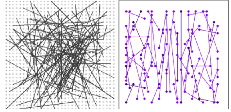
It turns out that tests are selected so that, on the one hand, the average value of these tests is as close as possible to 0.5, on the other hand, the correlation between different tests is minimal. And this is what we need. Compare how it was and how it became:



Fortunately, the ORB algorithm is implemented in the OpenCV library in the class cv :: ORB. I am using version 2.4.13. The class constructor takes the following parameters:

nfeatures - the maximum number of special points
scaleFactor is a multiplier for the pyramid of images, greater than one. A value of 2 implements the classic pyramid.
nlevels - the number of levels in the pyramid of images.
edgeThreshold is the number of pixels near the border of the image where special points are not detected.
firstLevel - leave zero.
WTA_K is the number of dots required for one descriptor element. If equal to 2, then compares the brightness of two randomly selected pixels. This is necessary.
scoreType - if 0, then Harris is used as a measure of the singularity, otherwise - the FAST measure (based on the sum of magnitudes of differences in brightness at points of a circle). The FAST measure is slightly less stable, but it works faster.
patchSize is the size of the neighborhood from which random pixels are selected for comparison. The code searches and compare the special points on two pictures, “templ.bmp” and “img.bmp”


If someone has helped to understand the essence of the algorithms, then everything is not in vain. All Habra.

Literature:

1. Fusing Points and Lines for High Performance Tracking
2. Machine learning for high-speed corner detection
3. Faster and better: a machine learning approach to corner detection
4. BRIEF: Binary Robust Independent Elementary Features
5. ORB: an alternative to SIFT or SURF