Polynomial regression model

In simple terms, the regression model in mathematical statistics is based on well-known data, which are pairs of numbers. The number of such pairs is predetermined. If we imagine that the first number in a pair is the value of the coordinate $$$x$ and the second is $$$y$ , then the set of such pairs of numbers can be represented on a plane in the Cartesian coordinate system as a set of points. These pairs of numbers are not taken randomly. In practice, as a rule, the second number depends on the first. To build a regression is to pick up such a line (more precisely, a function), which as closely as possible brings closer to itself (approximates) the set of the above points.

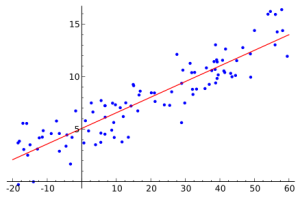
What is all this for? First of all, it is necessary to compile the so-called. forecasts. Often you need to know $$$y$ knowing only $$$x$ , if it differs from those X, on the basis of which the regression was built. I will give a simple example. There is a statistics of dependence of a person's height on his age on the basis of 100 different people studied. Thus, we have 100 pairs of numbers {age; growth}. At the same time, “growth” is a dependent quantity, and “age” is an independent one. Having built the regression model competently, we can “predict” growth with any certainty for any age value.

In practice, depending on the situation, linear, parabolic, power, and other types of functions are used in the construction of regression models. In the course of mathematical statistics, the linear regression model is most often considered. Sometimes the case is more complicated - a parabolic model. Making a generalization, it is easy to guess that linear and parabolic models are special cases of a more complex model - polynomial. To build a regression model is to find the parameters of the function that will appear in it. For linear regression, there are two parameters: a coefficient and a free term.

Polynomial regression can be applied in mathematical statistics when modeling trend components of time series. A time series is essentially a series of numbers that depend on time. For example, the average values ​​of air temperature by day over the past year, or enterprise income by months. The order of the simulated polynomial is estimated by special methods, for example, the criterion of the series. The goal of building a polynomial regression model in the time series domain is the same — forecasting.

To begin, consider the problem of polynomial regression in general. All reasoning is based on the generalization of reasoning in linear and parabolic regression problems. After these arguments, I will proceed to a special case - the consideration of this model for time series.

Let two series of observations be given. $$$x_i$ (independent variable) and $$$y_i$ (dependent variable) $$$i = \ overline {1, n}$ . The polynomial equation has the form

$$

$$y = \ sum \ limits_ {j = 0} ^ k b_jx ^ j, \ \ \ \ \ (1)$$

Where $$$b_j$ - the parameters of this polynomial, $$$j = \ overline {0, k}$ . Among them $$$b_0$ - free member. Find the least squares (OLS) method parameters $$$b_j$ this regression.

By analogy with linear regression, OLS is also based on minimizing the following expression:

$$

$$S = \ sum \ limits_ {i = 1} ^ n \ left (\ hat y_i-y_i \ right) ^ 2 \ to \ min \ \ \ \ \ (2)$$

Here $$$\ hat y_i$ - theoretical values, which are the values ​​of the polynomial (1) at the points $$$x_i$ . Substituting (1) into (2), we obtain

$$

$$S = \ sum \ limits_ {i = 1} ^ n \ left (\ sum_ {j = 0} ^ kb_jx_i ^ j-y_i \ right) ^ 2 \ to \ min.$$

Based on the necessary condition of the extremum function $$$(k + 1)$ variables $$$S = S (b_0, b_1, \ dots, b_k)$ we equate its partial derivatives to zero, i.e.

$$

$$S '_ {b_p} = 2 \ sum \ limits_ {i = 1} ^ nx_i ^ p \ left (\ sum \ limits_ {j = 0} ^ kb_jx_i ^ j-y_i \ right) = 0, \ \ \ p = \ overline {0, k}.$$

Dividing the left and right sides of each equality by 2, we open the second sum:

$$

$$\ sum \ limits_ {i = 1} ^ nx_i ^ p \ left (b_0 + b_1x_i + b_2x_i ^ 2 + \ dots + b_kx_i ^ k \ right) - \ sum \ limits_ {i = 1} ^ nx_i ^ py_i = 0 , \ \ \ p = \ overline {0, k}.$$

Opening brackets, we transfer in each $$$p$ th term last term with $$$y_i$ right and divide both parts into $$$n$ . As a result, we got $$$(k + 1)$ expressions forming a system of linear normal equations with respect to $$$b_p$ . It has the following form:

$$

$$\ left \ {\ begin {array} {l} b_0 + b_1 \ overline x + b_2 \ overline {x ^ 2} + \ dots + b_k \ overline {x ^ k} = \ overline y \\ b_0 \ overline x + b_1 \ overline {x ^ 2} + b_2 \ overline {x ^ 3} + \ dots + b_k \ overline {x ^ {k + 1}} = \ overline {xy} \\ b_0 \ overline {x ^ 2} + b_1 \ overline {x ^ 3} + b_2 \ overline {x ^ 4} + \ dots + b_k \ overline {x ^ {k + 2}} = \ overline {x ^ 2y} \\ ldots \ ldots \ ldots \ ldots \ ldots \ ldots \ ldots \ ldots \ ldots \ ldots \ ldots \ ldots \ ldots \\ b_0 \ overline {x ^ k} + b_1 \ overline {x ^ {k + 1}} + b_2 \ overline {x ^ {k + 2}} + \ dots + b_k \ overline {x ^ {2k}} = \ overline {x ^ ky} \ end {array} \ right. \ \ \ \ \ (3)$$

You can rewrite the system (3) in matrix form: $$$AB = C$ where

$$

$$A = \ left (\ begin {array} {ccccc} 1 & \ overline x & \ overline {x ^ 2} & \ ldots & \ overline {x ^ k} \\ \ overline x & \ overline {x ^ 2 } & \ overline {x ^ 3} & \ ldots & \ overline {x ^ {k + 1}} \\ \ overline {x ^ 2} & \ overline {x ^ 3} & \ overline {x ^ 4} & \ ldots & \ overline {x ^ {k + 2}} \\ \ vdots & \ vdots & \ vdots & \ ddots & \ vdots \\ \ overline {x ^ k} & \ overline {x ^ {k + 1} } & \ overline {x ^ {k + 2}} & \ ldots & \ overline {x ^ {2k}} \ end {array} \ right), \ \ B = \ left (\ begin {array} {c} b_0 \\ b_1 \\ b_2 \\\ vdots \\ b_k \ end {array} \ right), \ \ C = \ left (\ begin {array} {c} \ overline y \\ overline {xy} \\ \ overline {x ^ 2y} \\\ vdots \\\ overline {x ^ ky} \ end {array} \ right).$$

We now turn to the application of the above facts in the case of time series. Let given a time series $$$x_t$ where $$$t = \ overline {1, n}$ . Requires build polynomial trend of order $$$k$ which approximates a given time series as precisely as possible. As an independent variable $$$x$ we will take $$$t$ based on the definition of a time series. These X's are a series of natural numbers denoting a period of time. As $$$y$ time series values ​​are taken $$$x_t$ . In this case, it is clear that the values ​​of elements $$$a_ {ij}$ system matrices $$$A$ do not depend on $$$x_t$ . Since in the general case, obviously,

$$

$$a_ {ij} = \ overline {x ^ {i + j-2}} = \ frac1n \ sum \ limits_ {r = 1} ^ nx_r ^ {i + j-2},$$

then in the case of time series

$$

$$a_ {ij} = \ frac1n \ sum \ limits_ {r = 1} ^ nr ^ {i + j-2},$$

Where $$$i, j = \ overline {1, (k + 1)}.$

Items $$$c_j$ free vector matrixes $$$C$ generally obtained as

$$

$$c_j = \ overline {x ^ {j-1} y} = \ frac1n \ sum \ limits_ {r = 1} ^ nx_r ^ {j-1} y_r.$$

And in the case of time series

$$

$$c_j = \ frac1n \ sum \ limits_ {r = 1} ^ nr ^ {j-1} x_r,$$

Where $$$j = \ overline {1, (k + 1)}.$

Thus, having solved the system (3), we can find the desired parameters of the polynomial trend $$$b_0, \ dots, b_k.$

To fill the matrices of the system and to solve it, you can use one of the numerical methods for modeling the trend on the computer. In this case, the result of the calculation will be fairly accurate.

As a result, the trend component will look like:

$$

$$T_t = \ sum \ limits_ {i = 0} ^ kb_it ^ i, \ \ \ t = 0,1,2, \ dots.$$

It is also worth noting that the modeled trend component $$$T_t$ not defined only for current periods $$$[1; n]$ but also for future periods $$$t> n$ .

Immediately, I note that polynomial regression models only the trend component of the time series. The full time series model also implies other components, which is beyond the scope of this article.

In practice, I personally did not encounter time series with a polynomial trend order of more than 2. This explains the prevalence of linear and prabolic regression models as particular polynomial cases.