IGNG - incremental neural gas algorithm

When writing an article on the development of the anomaly detector, I implemented one of the algorithms called Incremental Growing Neural Gas.

AT ~~Soviet literature~~ In the Russian segment of the Internet, this topic is rather weakly covered, and only one article was found, and even then with the application of this algorithm.

So, what is the algorithm for incremental growing neural gas?

Introduction

IGNG, like GNG , is an adaptive clustering algorithm.
The algorithm itself is described in the article of Prudent and Ennaji for the year 2005 .

As with GNG, there are many data vectors. $X$ or generating function $f (t)$ which provides vectors from arbitrarily distributed data (parameter $t$ - time or sample number in the sample).

Additional restrictions on the data algorithm does not impose.
But, inside is very different from GNG.

This algorithm is also curious by the fact that it is slightly more accurate than GNG models neurogenesis .

Algorithm Description

The algorithm breaks a lot of data into clusters.
Compared to GNG, its advantage is a higher rate of convergence.

The ideas on which the algorithm is based:

Theory of adaptive resonance : “first, the nearest neuron is searched for, and if the difference does not exceed the threshold (“ vigilance parameter ”), the weights are corrected or, otherwise, the coordinate of the neuron is changed in the data space. If the threshold has not been overcome, new neurons are created, better approximating the value of the sample data.
Both connections and neurons have an age parameter (in GNG, only connections), which is initially zero, but increases with learning.
A neuron does not appear immediately: an embryo (or germinal neuron) first appears, whose age increases with each iteration until it matures. After training, only mature neurons participate in the classification .

Main loop

Work begins with a blank graph. Parameter $\ sigma$ initialized by the standard deviation of the training sample:

s i g m a = s q r t f r a c 1 N s u m l i m i t s_{i = 1}^{N} l e f t (x_{i} - b a r x r i g h t)^{2}

$\ sigma = \ sqrt {\ frac {1} {N} \ sum \ limits_ {i = 1} ^ N {\ left ({x_i - \ bar x} \ right) ^ 2}}$

Where: $\ bar x$ - the average between the coordinates of the sample.

The main loop at each step decreases the value. $\ sigma$ which is the proximity threshold, and calculates the difference between the previous level of clustering quality and the level that was obtained after clustering by the IGNG procedure .

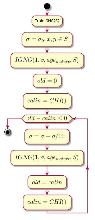
Chart code.

@startuml start :TrainIGNG(S); :<latex>\sigma = \sigma_S,x,y \in S</latex>; :<latex>IGNG(1, \sigma, age_{mature}, S)</latex>; :<latex>old = 0</latex>; :<latex>calin = CHI()</latex>; while (<latex>old - calin \leq 0</latex>) :<latex>\sigma=\sigma - \sigma / 10</latex>; :<latex>IGNG(1, \sigma, age_{mature}, S)</latex>; :<latex>old = calin</latex>; :<latex>calin = CHI()</latex>; endwhile stop @enduml

CHI is the Kalinsky-Kharabaza index, showing the quality of clustering:

C H I = f r a c B / (c - 1) W / (n - c)

$CHI = \ frac {B / (c - 1)} {W / (n - c)}$

Where:

$n$ - The number of data samples.
$c$ - the number of clusters (in this case, the number of neurons).
$B$ - matrix of internal dispersion (the sum of the squares of the distances between the coordinates of the neurons and the average for all data).
$W$ - matrix of external dispersion (the sum of squares of the distance between all data and the nearest neuron).

The larger the index value, the better, because if the difference between the indices after clustering and before it is negative, it is possible to assume that the index became positive and exceeded the previous one, i.e. clustering completed successfully.

IGNG procedure

This is the basic procedure of the algorithm.

It is divided into three mutually exclusive stages:

Neurons not found.
Found one that satisfies the conditions of the neuron.
Found two that satisfy the conditions of the neuron.

If one of the conditions passes, the other steps are not performed.

First, a neuron is searched for the best approaching sample data:

c_{1} = m i n (d i s t (x i, o m e g a_{c}))

$c_1 = min (dist (\ xi, \ omega_c))$

Here $dist (x_ \ omega, x_ \ xi)$ - the function of calculating the distance, which is usually the Euclidean metric .

If the neuron is not found, or it is too far from the data, i.e. does not meet the criterion of approximation $dist (\ xi, \ omega_c) \ leq \ sigma$ A new embryonic neuron is created with coordinates equal to the coordinates of the sample in the data space.

If the proximity test has passed, the second neuron is searched in a similar way and its proximity to the data sample is checked.
If the second neuron is not found, it is created.

If two neurons were found that satisfy the condition of proximity to the data sample, their coordinates are corrected by the following formula:

e p s i l o n (t) h_{c, c_{i}} = b e g i n c a s e s e p s i l o n_{b}, i f c = c_{i} e p s i l o n_{n}, i f i s c o n n e c t i o n b e t w e e n c = c_{i} 0, i n o t h e r w i s e c a s e e n d c a s e s

$\ epsilon (t) h_ {c, c_i} = \ begin {cases} \ epsilon_b, \, if \, c = c_i \\ \ epsilon_n, \, if \, is \, connection \, between \, c = c_i \\ 0, \, in \, otherwise \, case \ end {cases}$

D e l t a o m e g a_{c} = e p s i l o n (t) h_{c},_{c 1} p a r a l l e l x i - o m e g a_{c} p a r a l l e l o m e g a_{c} = o m e g a_{c} + D e l t a o m e g a_{c}

$\ Delta \ omega_c = \ epsilon (t) h_c, _ {c1} \ parallel \ xi - \ omega_c \ parallel \\ \ omega_c = \ omega_c + \ Delta \ omega_c$

Where:

$\ epsilon (t)$ - adaptation step.
$c_i$ - the number of the neuron.
$h_c, _ {c1}$ - Neuron Neighborhood Function $c$ with a neuron winner (in this case, it returns 1 for direct neighbors, 0 otherwise, because the adaptation step is for calculating $\ omega$ will be nonzero only for direct neighbors).

In other words, the coordinate (weight) of the winning neuron changes to $\ epsilon_b * \ Delta \ omega_ {i}$ , and all its direct neighbors (those connected with it by one edge of the graph) on $\ epsilon_n * \ Delta \ omega_ {i}$ where $\ omega_i$ - the coordinate of the corresponding neuron before the change.

Then a connection is created between the two winning neurons, and if it has already been created, its age will be reset.
The age of all other connections is increasing.

All connections whose age has exceeded a constant $age_ {max}$ are deleted.
After that, all isolated (those that have no connection with others) mature neurons are removed.

The age of the immediate neurons-neighbors of the neuron-winner increases.
If the age of any of the germinal neurons exceeds $age_ {mature}$ , it becomes a mature neuron.

The final graph contains only mature neurons.

The condition for the completion of the IGNG procedure below may be considered a fixed number of cycles.

The algorithm is shown below (the picture is clickable):

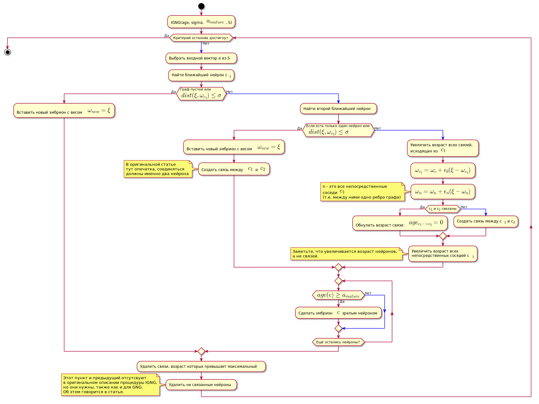
Chart code.

 @startuml skinparam nodesep 10 skinparam ranksep 20 start :IGNG(age, sigma, <latex>a_{mature}</latex>, S); while (  ) is () -[#blue]-> :   e  S; :   c<sub>1</sub>; if (  \n<latex>dist(\xi, \omega_{c_1}) \leq \sigma</latex>) then () :     <latex>\omega_{new} = \xi</latex>; else () -[#blue]-> :   ; if (     \n <latex>dist(\xi, \omega_{c_2}) \leq \sigma</latex>) then () :     <latex>\omega_{new} = \xi</latex>; :   <latex>c_1</latex>  <latex>c_2</latex>; note     ,      end note else () -[#blue]-> :   ,\n  <latex>c_1</latex>; :<latex>\omega_{c_1} = \omega_c + \epsilon_b(\xi - \omega_{c_1})</latex>; :<latex>\omega_n = \omega_n + \epsilon_n(\xi - \omega_n)</latex>; note n -     <latex>c_1</latex> (..     ) end note if (c<sub>1</sub>  c<sub>2</sub> ) then () :  : <latex>age_{c_1 -> c_2} = 0</latex>; else () -[#blue]-> :   c<sub>1</sub>  c<sub>2</sub>; endif :  \n  c<sub>1</sub>; note ,    ,   . end note endif repeat if (<latex>age(c) \geq a_{mature}</latex>) then () :  $<!-- math>c</math -->$  ; else () -[#blue]-> endif repeat while (  ?) endif : ,    ; :   ; note          IGNG,   ,     GNG.     . endnote endwhile () stop @enduml

Implementation

Network implementation is done in Python using the NetworkX graph library . Cutting out the code from the prototype in the previous article is given below. There is also a brief explanation of the code.

If someone is interested in the full code, here is the link to the repository .

Example of the algorithm:

Bulk code

 class NeuralGas(): __metaclass__ = ABCMeta def __init__(self, data, surface_graph=None, output_images_dir='images'): self._graph = nx.Graph() self._data = data self._surface_graph = surface_graph # Deviation parameters. self._dev_params = None self._output_images_dir = output_images_dir # Nodes count. self._count = 0 if os.path.isdir(output_images_dir): shutil.rmtree('{}'.format(output_images_dir)) print("Ouput images will be saved in: {0}".format(output_images_dir)) os.makedirs(output_images_dir) self._start_time = time.time() @abstractmethod def train(self, max_iterations=100, save_step=0): raise NotImplementedError() def number_of_clusters(self): return nx.number_connected_components(self._graph) def detect_anomalies(self, data, threshold=5, train=False, save_step=100): anomalies_counter, anomaly_records_counter, normal_records_counter = 0, 0, 0 anomaly_level = 0 start_time = self._start_time = time.time() for i, d in enumerate(data): risk_level = self.test_node(d, train) if risk_level != 0: anomaly_records_counter += 1 anomaly_level += risk_level if anomaly_level > threshold: anomalies_counter += 1 #print('Anomaly was detected [count = {}]!'.format(anomalies_counter)) anomaly_level = 0 else: normal_records_counter += 1 if i % save_step == 0: tm = time.time() - start_time print('Abnormal records = {}, Normal records = {}, Detection time = {} s, Time per record = {} s'. format(anomaly_records_counter, normal_records_counter, round(tm, 2), tm / i if i else 0)) tm = time.time() - start_time print('{} [abnormal records = {}, normal records = {}, detection time = {} s, time per record = {} s]'. format('Anomalies were detected (count = {})'.format(anomalies_counter) if anomalies_counter else 'Anomalies weren\'t detected', anomaly_records_counter, normal_records_counter, round(tm, 2), tm / len(data))) return anomalies_counter > 0 def test_node(self, node, train=False): n, dist = self._determine_closest_vertice(node) dev = self._calculate_deviation_params() dev = dev.get(frozenset(nx.node_connected_component(self._graph, n)), dist + 1) dist_sub_dev = dist - dev if dist_sub_dev > 0: return dist_sub_dev if train: self._dev_params = None self._train_on_data_item(node) return 0 @abstractmethod def _train_on_data_item(self, data_item): raise NotImplementedError() @abstractmethod def _save_img(self, fignum, training_step): """.""" raise NotImplementedError() def _calculate_deviation_params(self, distance_function_params={}): if self._dev_params is not None: return self._dev_params clusters = {} dcvd = self._determine_closest_vertice dlen = len(self._data) #dmean = np.mean(self._data, axis=1) #deviation = 0 for node in self._data: n = dcvd(node, **distance_function_params) cluster = clusters.setdefault(frozenset(nx.node_connected_component(self._graph, n[0])), [0, 0]) cluster[0] += n[1] cluster[1] += 1 clusters = {k: sqrt(v[0]/v[1]) for k, v in clusters.items()} self._dev_params = clusters return clusters def _determine_closest_vertice(self, curnode): """.""" pos = nx.get_node_attributes(self._graph, 'pos') kv = zip(*pos.items()) distances = np.linalg.norm(kv[1] - curnode, ord=2, axis=1) i0 = np.argsort(distances)[0] return kv[0][i0], distances[i0] def _determine_2closest_vertices(self, curnode): """Where this curnode is actually the x,y index of the data we want to analyze.""" pos = nx.get_node_attributes(self._graph, 'pos') l_pos = len(pos) if l_pos == 0: return None, None elif l_pos == 1: return pos[0], None kv = zip(*pos.items()) # Calculate Euclidean distance (2-norm of difference vectors) and get first two indexes of the sorted array. # Or a Euclidean-closest nodes index. distances = np.linalg.norm(kv[1] - curnode, ord=2, axis=1) i0, i1 = np.argsort(distances)[0:2] winner1 = tuple((kv[0][i0], distances[i0])) winner2 = tuple((kv[0][i1], distances[i1])) return winner1, winner2 class IGNG(NeuralGas): """Incremental Growing Neural Gas multidimensional implementation""" def __init__(self, data, surface_graph=None, eps_b=0.05, eps_n=0.0005, max_age=5, a_mature=1, output_images_dir='images'): """.""" NeuralGas.__init__(self, data, surface_graph, output_images_dir) self._eps_b = eps_b self._eps_n = eps_n self._max_age = max_age self._a_mature = a_mature self._num_of_input_signals = 0 self._fignum = 0 self._max_train_iters = 0 # Initial value is a standard deviation of the data. self._d = np.std(data) def train(self, max_iterations=100, save_step=0): """IGNG training method""" self._dev_params = None self._max_train_iters = max_iterations fignum = self._fignum self._save_img(fignum, 0) CHS = self.__calinski_harabaz_score igng = self.__igng data = self._data if save_step < 1: save_step = max_iterations old = 0 calin = CHS() i_count = 0 start_time = self._start_time = time.time() while old - calin <= 0: print('Iteration {0:d}...'.format(i_count)) i_count += 1 steps = 1 while steps <= max_iterations: for i, x in enumerate(data): igng(x) if i % save_step == 0: tm = time.time() - start_time print('Training time = {} s, Time per record = {} s, Training step = {}, Clusters count = {}, Neurons = {}, CHI = {}'. format(round(tm, 2), tm / (i if i and i_count == 0 else len(data)), i_count, self.number_of_clusters(), len(self._graph), old - calin) ) self._save_img(fignum, i_count) fignum += 1 steps += 1 self._d -= 0.1 * self._d old = calin calin = CHS() print('Training complete, clusters count = {}, training time = {} s'.format(self.number_of_clusters(), round(time.time() - start_time, 2))) self._fignum = fignum def _train_on_data_item(self, data_item): steps = 0 igng = self.__igng # while steps < self._max_train_iters: while steps < 5: igng(data_item) steps += 1 def __long_train_on_data_item(self, data_item): """.""" np.append(self._data, data_item) self._dev_params = None CHS = self.__calinski_harabaz_score igng = self.__igng data = self._data max_iterations = self._max_train_iters old = 0 calin = CHS() i_count = 0 # Strictly less. while old - calin < 0: print('Training with new normal node, step {0:d}...'.format(i_count)) i_count += 1 steps = 0 if i_count > 100: print('BUG', old, calin) break while steps < max_iterations: igng(data_item) steps += 1 self._d -= 0.1 * self._d old = calin calin = CHS() def _calculate_deviation_params(self, skip_embryo=True): return super(IGNG, self)._calculate_deviation_params(distance_function_params={'skip_embryo': skip_embryo}) def __calinski_harabaz_score(self, skip_embryo=True): graph = self._graph nodes = graph.nodes extra_disp, intra_disp = 0., 0. # CHI = [B / (c - 1)]/[W / (n - c)] # Total numb er of neurons. #ns = nx.get_node_attributes(self._graph, 'n_type') c = len([v for v in nodes.values() if v['n_type'] == 1]) if skip_embryo else len(nodes) # Total number of data. n = len(self._data) # Mean of the all data. mean = np.mean(self._data, axis=1) pos = nx.get_node_attributes(self._graph, 'pos') for node, k in pos.items(): if skip_embryo and nodes[node]['n_type'] == 0: # Skip embryo neurons. continue mean_k = np.mean(k) extra_disp += len(k) * np.sum((mean_k - mean) ** 2) intra_disp += np.sum((k - mean_k) ** 2) return (1. if intra_disp == 0. else extra_disp * (n - c) / (intra_disp * (c - 1.))) def _determine_closest_vertice(self, curnode, skip_embryo=True): """Where this curnode is actually the x,y index of the data we want to analyze.""" pos = nx.get_node_attributes(self._graph, 'pos') nodes = self._graph.nodes distance = sys.maxint for node, position in pos.items(): if skip_embryo and nodes[node]['n_type'] == 0: # Skip embryo neurons. continue dist = euclidean(curnode, position) if dist < distance: distance = dist return node, distance def __get_specific_nodes(self, n_type): return [n for n, p in nx.get_node_attributes(self._graph, 'n_type').items() if p == n_type] def __igng(self, cur_node): """Main IGNG training subroutine""" # find nearest unit and second nearest unit winner1, winner2 = self._determine_2closest_vertices(cur_node) graph = self._graph nodes = graph.nodes d = self._d # Second list element is a distance. if winner1 is None or winner1[1] >= d: # 0 - is an embryo type. graph.add_node(self._count, pos=copy(cur_node), n_type=0, age=0) winner_node1 = self._count self._count += 1 return else: winner_node1 = winner1[0] # Second list element is a distance. if winner2 is None or winner2[1] >= d: # 0 - is an embryo type. graph.add_node(self._count, pos=copy(cur_node), n_type=0, age=0) winner_node2 = self._count self._count += 1 graph.add_edge(winner_node1, winner_node2, age=0) return else: winner_node2 = winner2[0] # Increment the age of all edges, emanating from the winner. for e in graph.edges(winner_node1, data=True): e[2]['age'] += 1 w_node = nodes[winner_node1] # Move the winner node towards current node. w_node['pos'] += self._eps_b * (cur_node - w_node['pos']) neighbors = nx.all_neighbors(graph, winner_node1) a_mature = self._a_mature for n in neighbors: c_node = nodes[n] # Move all direct neighbors of the winner. c_node['pos'] += self._eps_n * (cur_node - c_node['pos']) # Increment the age of all direct neighbors of the winner. c_node['age'] += 1 if c_node['n_type'] == 0 and c_node['age'] >= a_mature: # Now, it's a mature neuron. c_node['n_type'] = 1 # Create connection with age == 0 between two winners. graph.add_edge(winner_node1, winner_node2, age=0) max_age = self._max_age # If there are ages more than maximum allowed age, remove them. age_of_edges = nx.get_edge_attributes(graph, 'age') for edge, age in iteritems(age_of_edges): if age >= max_age: graph.remove_edge(edge[0], edge[1]) # If it causes isolated vertix, remove that vertex as well. #graph.remove_nodes_from(nx.isolates(graph)) for node, v in nodes.items(): if v['n_type'] == 0: # Skip embryo neurons. continue if not graph.neighbors(node): graph.remove_node(node) def _save_img(self, fignum, training_step): """.""" title='Incremental Growing Neural Gas for the network anomalies detection' if self._surface_graph is not None: text = OrderedDict([ ('Image', fignum), ('Training step', training_step), ('Time', '{} s'.format(round(time.time() - self._start_time, 2))), ('Clusters count', self.number_of_clusters()), ('Neurons', len(self._graph)), (' Mature', len(self.__get_specific_nodes(1))), (' Embryo', len(self.__get_specific_nodes(0))), ('Connections', len(self._graph.edges)), ('Data records', len(self._data)) ]) draw_graph3d(self._surface_graph, fignum, title=title) graph = self._graph if len(graph) > 0: draw_graph3d(graph, fignum, clear=False, node_color=(1, 0, 0), title=title, text=text) mlab.savefig("{0}/{1}.png".format(self._output_images_dir, str(fignum))) #mlab.close(fignum)

Source: https://habr.com/ru/post/414209/

All Articles