Today we will talk about the most important features of PostgreSQL 11. Why only about them - because not everyone needs some of the features, so we stopped at the most popular ones.
Content

JIT compilation
In PostgreSQL, JIT compilation has finally appeared, that is, compiling requests into binary code. To do this, you need to compile PostgreSQL with support for JIT compilation
(Compile time 1 (--with-llvm)) . At the same time, the machine must have an LLVM version not lower than 3.9.
What can JIT accelerate?
- Queries with the WHERE clause, that is, everything that comes after this keyword. This is not always necessary, but the opportunity is useful.
- Calculation of the target list (target list): in the terminology of PostgreSQL, this is all that is between select and from.
- Aggregates.
- Transformation of record from one type to another (Projection). For example, when you apply join to two tables and the result is a new tuple containing fields from both tables.
- Tuple deforming. One of the problems of any database, at least, lower case, relational, is how to get the field from the disk record. After all, there may be null, they have different entries, and in general, this is not the cheapest operation.
Compile time 2 means that JIT is not used. In PostgreSQL, there is a moment of scheduling a request when the system decides what is worth JIT'it and what is not worth it. At this point, it JIT'and further executor performs as it is.
JIT is made pluggable. By default it works with LLVM, but you can plug in any other JIT.
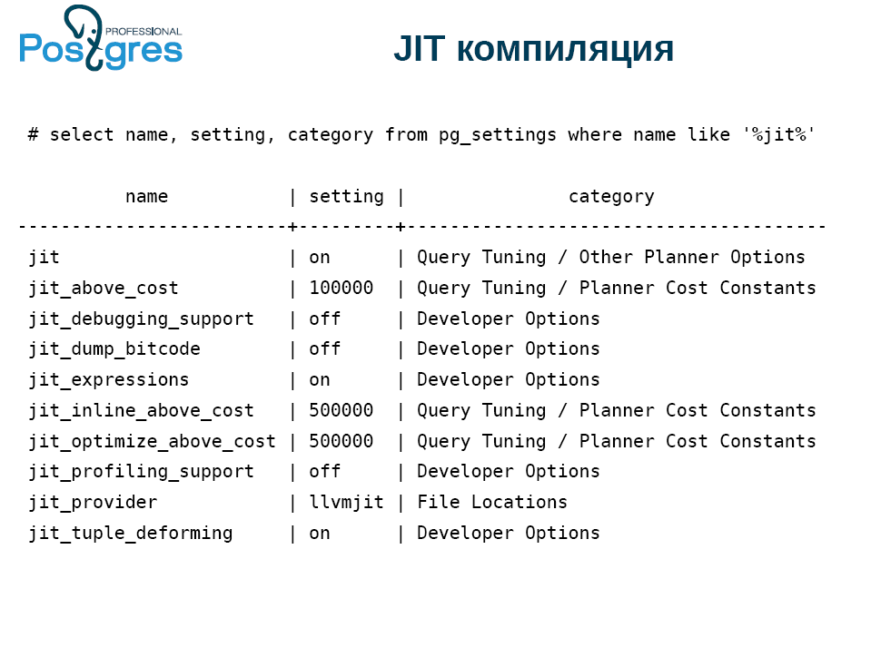
If you compiled PostgreSQL without JIT support, the very first setting does not work. Implemented options for developers, there are settings for individual JIT functions.
The next subtle point is associated with jit_above_cost. JIT itself is not free. Therefore, PostgreSQL by default deals with JIT optimization if the cost of the request exceeds 100 thousand conditional parrots, in which explain, analyze and so on is measured. This value is chosen at random, so pay attention to it.
But not always after turning on the JIT immediately everything works. Usually, everyone starts experimenting with JIT using the select * from table where id = 600 query and it doesn't work. Probably, it is necessary to somehow complicate the request, and then everyone generates a giant base and compose the request. As a result, PostgreSQL rests on the capacity of the disk, it lacks the capacity of common buffers or caches.
Here is a completely abstract example. There are 9 null fields with different frequencies so that you can notice the effect of tuple deforming.
select i as x1,
case when i % 2 = 0 then i else null end as x2,
case when i % 3 = 0 then i else null end as x3,
case when i % 4 = 0 then i else null end as x4,
case when i % 5 = 0 then i else null end as x5,
case when i % 6 = 0 then i else null end as x6,
case when i % 7 = 0 then i else null end as x7,
case when i % 8 = 0 then i else null end as x8,
case when i % 9 = 0 then i else null end as x9
into t
from generate_series(0, 10000000) i;

vacuum t;
analyze t;
PostgreSQL has a lot of opportunities, and to see the benefits of JIT, turn off the first two lines, so as not to interfere, and reset thresholds.
set max_parallel_workers=0;
set max_parallel_workers_per_gather=0;
set jit_above_cost=0;
set jit_inline_above_cost=0;
set jit_optimize_above_cost=0;
Here is the request itself:
set jit=off;
explain analyze
select count(*) from t where
sqrt(pow(x9, 2) + pow(x8,2)) < 10000;

set jit=on;
explain analyze
select count(*) from t where
sqrt(pow(x9, 2) + pow(x8,2)) < 10000;
And here is the result:
Planning Time: 0.71 ms
Execution Time: 1986.323 ms

VS

Planning Time: 0.060 ms
JIT:
Functions: 4
Generation Time: 0.911 ms
Inlining: true
Inlining Time: 23.876 ms
Optimization: true
Optimization Time: 41.399 ms
Emission Time: 21.856 ms
Execution Time: 949.112 ms
JIT helped speed up the request in half. Planning time is about the same thing, but this is most likely a consequence of the fact that PostgreSQL has cached something, so do not pay attention to it.
If you add up, then the JIT compilation took about 80 ms. Why is JIT not free? Before you run the query, you need to compile it, and this also takes time. And three orders of magnitude more than planning. Not a cheap pleasure, but it pays off due to the duration of the performance.
This is how JIT can be used, although it does not always benefit.
Sectioning
If you paid attention to partitioning in PostgreSQL, then you probably noticed that it was made there for a tick. The situation improved somewhat in version 10, when a declarative declaration of partitions (sections) appeared. On the other hand, everything inside remained the same and worked about the same as in previous versions, that is, it was bad.
In many ways, this problem was solved by the pg_pathman module, which allowed working with sections and rather optimally cutting them off at run time.
In version 11, partitioning is significantly improved:
- First, the partition table can have a primary key, which must include the partition key. In fact, this is either a semi-primary key, or a primary semi-key. Unfortunately, it is impossible to make a foreign key on it. I hope this will be corrected in the future.
- Also now it is possible to partition not only by range, but also by list and hash. The hash is quite primitive, for it takes the rest of the expression.
- When updating the line is moved between sections. Previously, it was necessary to write a trigger, but now it is done automatically.
The big question is: how many sections can you have? Honestly, with a large number of sections (thousands and tens of thousands), the feature works poorly. Pg_pathman does better.
Also made sections by default. Again, pg_pathman can be used to automatically create sections, which is more convenient. Here in the section everything that could not be shoved is dumped. If in a real system to do this by default, then after some time you get such a mess, which you then rake.
PostgreSQL 11 can now optimize partitioning if two tables are joined by a partitioning key, and partitioning schemes are the same. This is controlled by a special parameter that is turned off by default.
You can calculate the units for each section separately, and then summarize. Finally, you can create an index on the parent partitioned table, and then local indexes will be created on all the tables that are connected to it.
In the “What's New” section, a wonderful thing is mentioned - the ability to drop sections when executing a query. Let's check how it works. It turned out this table:

We make a type and a table of two columns with a primary key, with a bigserial column, insert data. Create a second table that will be partitioned and will be a copy of the first. Add the primary key to the partitioned table.
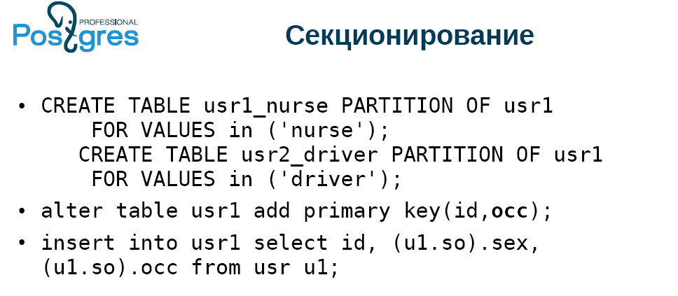
The table will consist of two types of records: “nanny women” and “male drivers”. And there will be one female driver. We make two sections, divide by the list, add the primary key and insert all the data from the table in which all this is generated. The result was completely uninteresting:

Pay attention to the request. We select everything from a non-partitioned table, connect it to a partitioned table. Take a small piece and choose only one type, they go through one. We indicate that the column ac should have one value. It turns out a sample of solid drivers.
During execution, we specifically disable paralleling, because by default PostgreSQL 11 very actively parallels more or less complex queries. If we look at the execution plan (explain analyze), it can be seen that the system has put the data in both sections: in the nanny, and in the drivers, although the nanny was not there. There were no calls to the buffer. Time spent, condition used, although PostgreSQL could figure it all out. That is, the ad partition elimination immediately does not work. Perhaps in the following assemblies this will be corrected. In this case, the pg_pathman module in this case works without problems.
Indices
- Bid optimization in monotonous order, i.e. b-tree. Everyone knows that when you insert monotonously growing data, it is not very fast. Now PostgreSQL is able to specifically cache the leaf page and not pass to insert all the way from the root. This significantly speeds up the work.
- In the PostgreSQL 10 version, the hash index can be used because it started using WAL (proactive write log). We used to get the value, unlock the page, return the value. For the next value, it was necessary to block the page again, return, unlock, and so on. Now hash began to work much faster. It allows you to block a page from a hash index at a time, retrieve all values from there and unlock it. This is now implemented for HASH, GiST and GIN. In the future, this will probably be implemented for SP-GiST. And for BRIN with its min / max logic, this cannot be done in principle.
- If earlier you built functional indexes, then HOT update (Heap Only Tuple) was effectively disabled. When an entry is updated in PostgreSQL, a new copy is actually created, and this requires inserting into all indexes that are in the table so that the new value points to a new tuple. Such optimization has been implemented for quite a long time: if the update does not change the fields that are not included in the indexes, and there is free space on the same page, then the indexes are not updated, and in the old version of tuple there is a pointer to the new version. This makes it possible to somewhat reduce the problem with updates. However, this optimization did not work at all if you have functional indexes. In PostgreSQL 11, it began to work. If you built a functional index and update the tuple, which does not change what the functional index depends on, then the HOT update will work.
Covering indexes
This functionality was implemented by PostgresPro three years ago, and all this time PostgreSQL tried to add it. The covering indexes mean that you can add additional columns to the unique index, directly into the index tuple.
What for? Everyone loves the index-only scan for fast work. To do this, build conditionally "covering" indices:
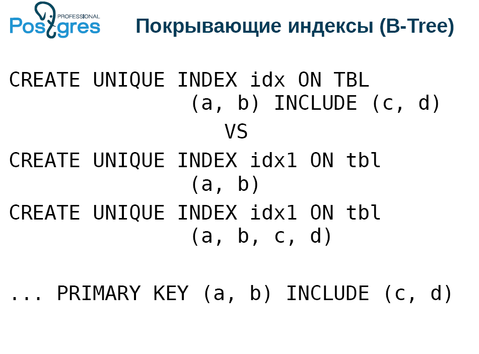
But it is necessary to preserve the uniqueness. Therefore, two indices are built, narrow and wide.
The disadvantage is that when you apply vacuum, insert, or update to the table, you need to update both indices without fail. So inserting into the index is a slow operation. And the covering index will allow to manage only one index.
True, he has some limitations. More precisely, the benefits that may not be immediately clear. The columns c and d in the first create index do not have to be scalar types for which the b-tree index is defined. That is, they do not necessarily have a more-less comparison. These can be points or polygons. The only thing is that a tuple must be less than 2.7 Kb, because there is no toasting in the index, but there you can fit what is impossible to compare.
However, inside the index with these guaranteed covered columns, no computation is performed during the search. This should be done by the filter that stands above the index. On the one hand, why not calculate it inside the index, on the other hand, it is an extra function call. But everything is not as scary as it seems.
Well, in addition, you can add these covered columns to the primary key.
SP GiST
This index is used by very few people because it is quite specific. Nevertheless, the opportunity to store in it is not exactly what they inserted. This refers to lossy - index, compression. As an example, take the polygons. Instead, an index is placed in the bounding box, that is, the minimum rectangle that contains the desired polygon. In this case, we represent a rectangle as a point in four-dimensional space, and then we work with the classic quad3, in four-dimensional space.
Also for SP-GiST introduced the operation "prefix search". It returns true if one line is prefixed by another. They introduced this for a reason, but for the sake of such a request with support for SP-GiST.
SELECT * FROM table WHERE c ^@ „abc“In b-tree there is a limit of 2.7 Kb for the entire line, while SP-GiST does not have such a limit. True, PostgreSQL has a limitation: one value cannot exceed 1 GB.
Performance
- A bitmap index only scan appeared . It works just like the classic index only scan, except that it cannot guarantee any order. Therefore, it is applicable only for some aggregates of the type count (*), because bitmap is not able to transfer the fields from the index to the executor. He can only report the fact of recording that satisfies the conditions.
- The next innovation is the update of Free Space Map (free page maps) during the application of vacuum . Unfortunately, none of the developers of systems working with PostgreSQL think that it is necessary to delete at the end of the table, otherwise holes appear, unallocated space. In order to track this, we implemented FSM, which allows us not to enlarge the table, but to insert a tuple into the voids. Previously, this was done using vacuum, but at the end. And now vacuum is able to do this in the process, and in high-load systems it helps to keep the size of the table under control.
- Ability to skip index scans during vacuum execution . The fact is that all PostgreSQL indexes, according to the theory of databases, are called secondary. This means that indexes are stored away from the table, pointers lead to it from them. Index only scan allows you not to make this jump along the signs, but to take it directly from the index. But vacuum, which deletes records, cannot look at them in the index to decide whether to delete or not, simply because there is no such data in the index. Therefore, vacuum is always executed in two passes. First goes through the table and finds out what he needs to delete. Then it goes to the indexes associated with this table, deletes the records that refer to what was found, returns to the table and deletes what was collected. And the stage of circulation in the indices is not always required.
If since the last vacuum there was no delete or update, then you do not have dead entries, they do not need to be deleted. In this case, the index can not go. There are additional subtleties, b-tree does not delete its pages immediately, but in two passes. Therefore, if you delete a lot of data in the table, then vacuum should be done. But if you want to free up space in the indexes, then vacuum twice.
Someone wonders, what is this table, in which there was no delete or update? In fact, many are dealing with this, just do not think. These are append only tables where logs are added, for example. In them, the removal is extremely rare. And it greatly saves the duration of vacuum / autovacuum, reduces the load on the disk, the use of caches and so on. - Simultaneous commit of competitive transactions . This is not an innovation, but an improvement. PostgreSQL now detects that it will commit now, and delays the commit of the current transaction, waiting for the remaining commits. Please note that this feature has little effect if you have a small server with 2-4 cores.
- postgres_fdw (Foreign Data Wrappers) . FDW is a way to connect an external data source so that it looks like a real post-Congress one. postgres_fdw allows you to connect a table from a neighboring instance to your copy, and it will look almost like a real one. Now removed one of the restrictions for update and delete. Often, PostgreSQL can guess that you need to send non-raw data. The way to perform a query with join is quite simple: we execute it on our machine, pull out a table from an instance using FDW, find out the id primary key that needs to be deleted, and then use update and / or delete, that is, the data we go back and forth . Now it is possible to do it. Of course, if the tables are on different machines, it is not so easy, but FDW allows the remote machine to perform the operations, and we just waited.
- toast_tuple_target . There are situations when the data is slightly beyond the limits, after which it is necessary toast'it, but at the same time toast of such values is not always pleasant. Suppose you have a limit of 90 bytes, and you need to fit 100. You have to get toast for 10 bytes, add them separately, then when you select this field, you need to refer to the toast index, find out where the necessary data lie, go to the toast table, collect and give away.
Now, using tweaking, you can change this behavior for the entire database or for a separate table, so that such small overruns do not require the use of toast. But you have to understand what you are doing, without this nothing happens.
WAL
- WAL (Write ahead log) is a proactive write log. WAL segment size is now set in initdb. Thank God, not when compiling.
- Also, the logic has changed. Previously, the set of WAL-segments was saved from the moment of the penultimate checkpoint, and now from the last one. This allows you to significantly reduce the amount of stored data. But if you have a database of 1 TB and TPS = 1, that is, one request per second, then you will not see the difference.
Backup and Replication
- Truncate appeared in logical replication . It was the last of the DML operations that was not reflected in logical replication. Now reflected.
- A message about prepare appeared in logical replication . Now you can catch the prepare transaction, a two-phase commit in logical replication. This is implemented for the construction of clusters - heterogeneous, homogeneous, shardirovanny and not shardirovannyh, multimasters and so on.
- The exception from pg_basebackup is temporary and unlogged tables . Many complained that pg_basebackup includes the listed tables. And excluding them, we reduce the size of the backup. But provided that you use temporary and unlogged tables, otherwise this option will be useless to you.
- Checksum control in stream replication (for tables) . This allows you to understand what happened to you with the replica. While the function is implemented only for tables.
- There was a promotka of positions replication slot . As always, you can only wind forward in time, back only if there is a WAL. Moreover, you need to understand very well what you are doing with this and why. In my opinion, this is more a development option, but those who use logical replication for some exotic applications can rejoice at it.
For DBA
- Alter table, add column, not null default X , write the entire table. For this there is a small fee: the default value is stored separately. If you raise a tuple and require this column, PostgreSQL has to go along an additional encoding path in order to pull out a temporary value, substitute it in a tuple and give it to you. However, you can live with it.
- Vacuum / analyze . Previously, it was possible to apply vacuum or analyze only to the entire database or one table. Now it is possible to do this to multiple tables, with one command.
Parallel execution
- Parallel construction of b-tree indexes . In version 11, it became possible to embed b-tree indexes into several workers. If you have a really good car, a lot of disks and a lot of cores, then you can build indexes in parallel, it promises a noticeable increase in performance.
- Parallel hash connection using a shared hash table for performers . , -. , . - , . .
- , union, create table as, select create materialized view!
- - (limit) . .
:
alter table usr reset (parallel_workers)
create index on usr(lower((so).occ)) — 2
alter table usr set (parallel_workers=2)
create index on usr(upper((so).occ)) — 1.8
parallel worker. . 16 4 ( ) 2 ., — 1,8 . , , . , .
:
explain analyze
select u1.* from usr u, usr1 u1 where
u.id=u1.id+0
, . , user — , . . , , .
, PostgreSQL 11 .

1425 , 1,5 . 1,4 . 2 . , 9.6 : 1 — 1 ., 2 1 . , 10 tuple. 11 . : user, batch, x-scan append .
:
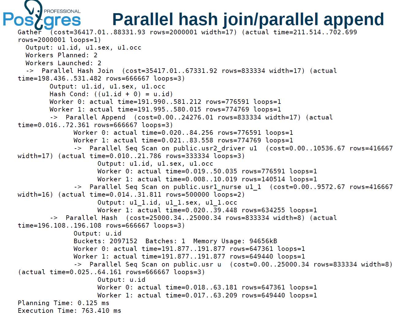
. 211 , 702 . , 510 1473. , 2 .
parallel hash join. . — 4. , .
parallel index scan . batch . What does this mean? hash join, . user . , parallel hash, .
1 . , OLAP-, OLTP . OLTP , .
.
- . , . , «» «», index scan, . (highly skewed data), , . . , , .
- «», .
Window-
SQL:2011, .
, , . , , , , , .
websearch, . , . , .
# select websearch_to_tsquery('dog or cat');
----------------------
'dor' | 'cat'
# select websearch_to_tsquery('dog -cat');
----------------------
'dor' & !'cat'
# select websearch_to_tsquery('or cat');
----------------------
'cat'
— dog or cat — . Websearch . | , . “or cat”. , . websearch “or” . , -, .
Websearch — . : , . , .
Json(b)
10- , 11- . json json(b), tsvector. ( json(b)) - . , , , bull, numeric, string, . .
# select jsonb_to_tsvector
('{"a":"texts", "b":12}', '"string"');
-------------------
'text':1
# select jsonb_to_tsvector
('{"a":"texts", "b":12}', '["string", "numeric"]');
-------------------
'12':3 'text':1
json(b), . , , , .
PL/*
.
CREATE PROCEDURE transaction_test1()
LANGUAGE plpgsql
AS $$
BEGIN
FOR i IN 0..9 LOOP
INSERT INTO test1 (a) VALUES (i);
IF i % 2 = 0 THEN
COMMIT;
ELSE
ROLLBACK;
END IF;
END LOOP;
END
$$;
CALL transaction_test1();
call, , . . . select, insert .
, , PostgreSQL . Perl, Python, TL PL/pgSQL. Perl sp begin, .
PL/pgSQL : , .
pgbench
pgbench ICSB bench — , , . if, , . case, - .
--init-steps , , .
random-seed. zipfian- . / — , . - , , - , .
, , - .
PSQL
, PSQL, . exit quit.
- — copy, 2 32 . copy : 2 32 - . , 2 31 2 32 copy . 64- , 2 64 .
- POSIX : NaN 0 = 1 1 NaN = 1.