Determination of the ballistic-temporal characteristics of the motion of the center of mass of a parachutist, landed from an airplane

Introduction

To determine the ballistic-temporal characteristics of the movement of the center of mass of the parachutist, one has to choose a simplified mathematical model that is quite accessible for analytical research and at the same time retains the most characteristic features of the original object.

To build simplified mathematical models of the movement of a parachutist, analysis, definition, systematization of permanent and temporary parameters are carried out.

Currently there are no regular and sufficiently substantiated methods for constructing nonlinear mathematical models; however, for solving particular problems, with proper preparation of initial systems of nonlinear differential equations, numerical methods for solving them can yield quite adequate results.

The purpose of this publication is to compile and numerically solve systems of differential equations that describe all stages of a parachutist’s movement, landed from an airplane, taking into account the effect of a change in altitude and temperature on the mass density of the air.

Ballistic-temporal characteristics of the movement of the parachutist

The permanent and limited variable parameters include:

H - the height of the parachutist;
V0 - the speed of the aircraft;
k - weight, height parachutist;
g - gravitational acceleration;
ρ is the air density;
T is the air temperature.

Temporary (variable) parameters include:

tn is the landing time
w - wind speed;
V is the speed of the parachutist;
u is the speed of the ascending (descending) flows;
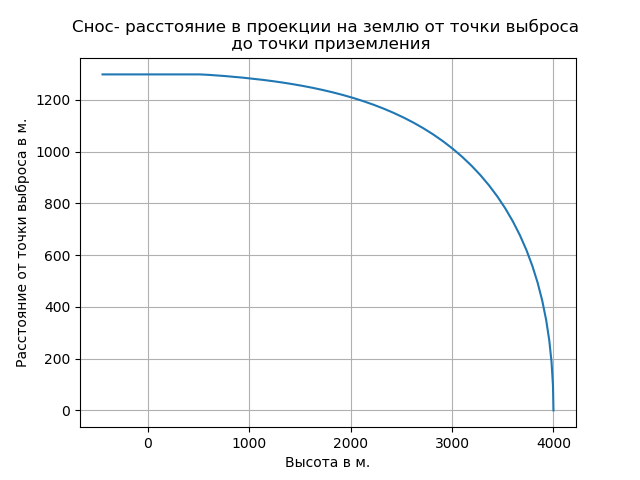
d - drift (distance from the projection on the ground of the point of ejection to the point of landing)
C is the drag coefficient of the object to be landed;
F - midsection of the object to be landed.

Jump stages

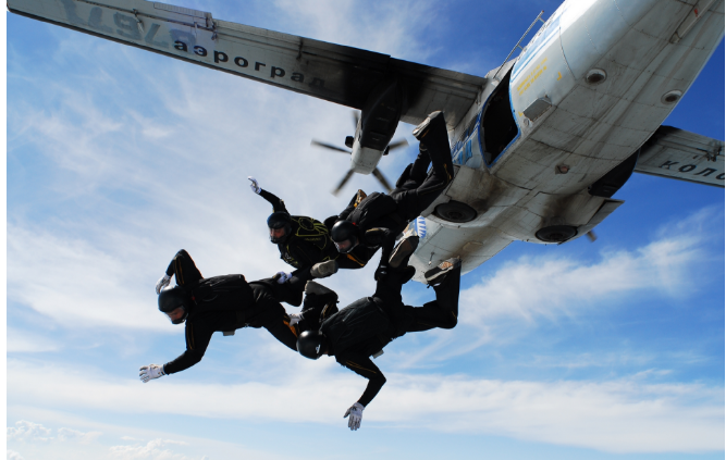
The first stage is a free fall after separation from the aircraft:

The second stage is a descent on a stabilizing parachute:

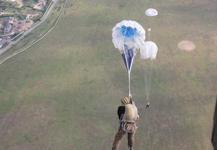
The main property of the stabilizing parachute is the stabilization of the parachutist in the position most convenient for the operation of the main parachute.

The third stage is the filling of the main parachute dome:

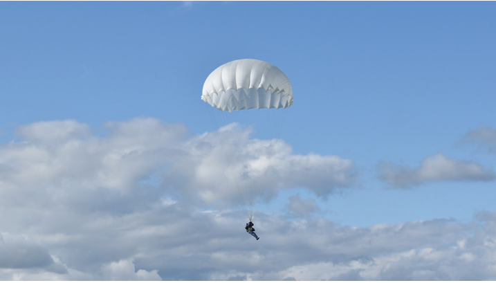
The fourth stage is a descent on an open parachute:

Drawing up a system of differential equations for all stages of a parachute jump

We choose a fixed coordinate system OXY centered at the point of emission O. The axis OX coincides with the direction of the horizontal component of the velocity of the aircraft. The axis OY is directed vertically upwards in the direction opposite to the vertical speed of a parachutist.

We will assume that the parachutist’s movement is flat and occurs in the OXY plane. This model of a jump can be considered as a model of a jump in calm weather without taking into account the influence of the wind.

We believe that the parachutist, besides the weight, is affected by the force of air resistance, which is proportional to the square of the speed of the parachutist:

,
Where:

- air density, - drag coefficient, F - midsection of the body.

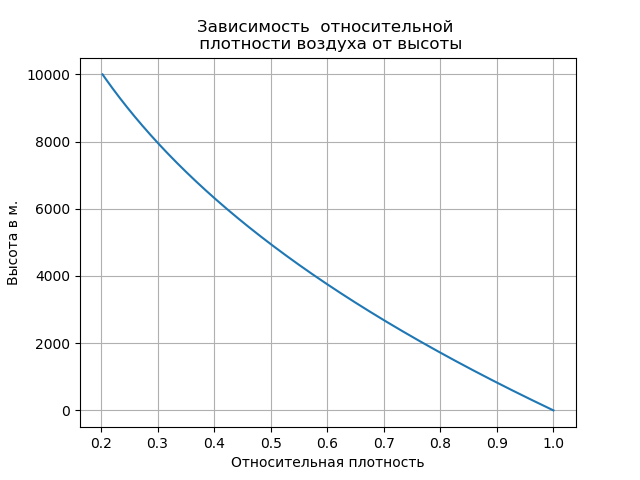
With increasing altitude, the air temperature changes:

The minimum temperature is reached already at an altitude of 10 km. and is -55 ° C. Air density also depends on pressure. Therefore, when calculating the parachute jump ballistics, it is convenient to use the following formula for determining air density [1]:

,
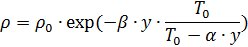
Where

K / m;

- temperature at sea level; y - height in m;

- air density at y = 0;

Listing

# -*- coding: utf8 -*- from numpy import* import matplotlib.pyplot as plt beta=1.25*10**-4 alfa=6.5*10**-3 T0=300 y=arange(0,10000,1) x=[exp(-beta*w*T0/(T0-alfa*w)) for w in y] plt.title("  \n    ") plt.plot(x,y) plt.ylabel('  .') plt.xlabel(' ') plt.grid(True) plt.show()

In practice, calculations for the value of the mid-section take the square of growth; C value is found from the table [2]:

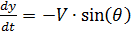
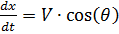
Through θ denotes the angle of the trajectory. Under the assumptions made for the components

velocity vector V we have:

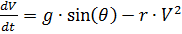
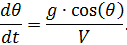
Dividing by m the left and right sides of the equations of the resulting system and denoting

through r, we get:

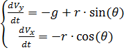
(one)

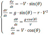
We write the equations of motion of the parachutist in the form of a system of differential equations for the functions V, θ, y (t), x (t).

Considering that:

,
and differentiating by time the ratio:

, taking into account the system of equations (1), we obtain:

.

Thus, under the initial conditions:

we have the following system of differential equations:

Numerical solution of the system of differential equations (2) by means of Python

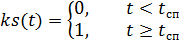
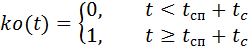
To solve (2), we rewrite it in the following form, by introducing the resistance forces stabilizing in time and air density

and main

parachutes, respectively, multiplied by the time control functions ks (t) and ko (t):

,

Where:

–Free-fall time parachutist;

- the operation time of the stabilization parachute before the opening of the main one.

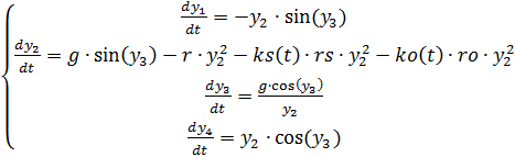
(3)

Full listing of the program, adjusted for changes in air density

 # -*- coding: utf8 -*- from numpy import* from scipy.integrate import odeint import matplotlib.pyplot as plt g=9.81#   /2 rou0=1.29#  /3 Cp=0.3#    Cpar=0.75#     mp=120#    100+20=120 . s=0.8#   2 ss=1.5#   2 Cpars=0.35#     S=70#   2 tsp=40#    c. tssp=3 #      c. tpr=210#     . h=4000.0#    . V0=100.0#    / beta=1.25*10**-4 alfa=6.5*10**-3 T0=300 def ks(t): if t<= tsp: z=0 else: z=1 return z def ko(t): if t<= tsp+tssp: z=0 else: z=1 return z def f(y,t): y1,y2,y3,y4=y rou=rou0*exp(-beta*y1*T0/(T0-alfa*y1)) rp=0.5*Cp*rou*s/mp rpars=0.5*Cpars*rou*ss/mp rpar=0.5*Cpar*rou*S/mp return [-y2*sin(y3),g*sin(y3)-rp*(y2**2)-ko(t)*rpar*(y2**2)-ks(t)*rpars*(y2**2),g*cos(y3)/y2,y2*cos(y3)] t=arange(0,tpr,1) y0=[h,100,0,0] [y1,y2,y3,y4]=odeint(f, y0,t, full_output=False).T plt.figure() plt.title('     : %s .. \n   : %s /. \n   : %s /'%(h,V0,round(y2[tpr-tsp-tssp],0))) plt.plot(y1,y2*sin(y3),label='  .: %s c. \n     : %s . \n     : %s . '%(tsp,tssp,tpr-tsp-tssp)) plt.xlabel('  .') plt.ylabel('   /') plt.legend(loc='best') plt.grid(True) plt.figure() plt.title("-         \n   ") plt.plot(y1,y4) plt.xlabel('  .') plt.ylabel('     .') plt.grid(True) plt.figure() plt.title("     ") plt.plot(t,y2*sin(y3)) plt.xlabel('  .') plt.ylabel('   /.') plt.grid(True) plt.show()

We get:

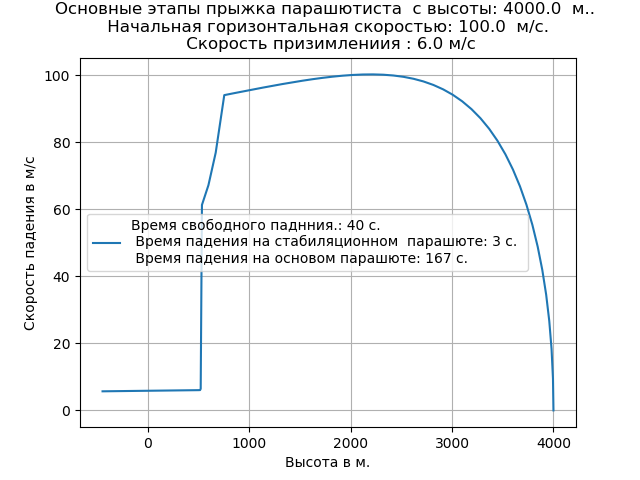
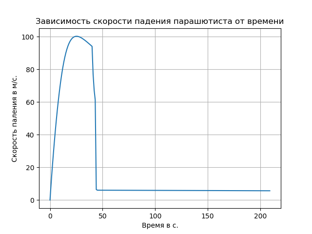
Accounting for rarefaction of air led to an increase in the speed of free fall and changed the nature of the trajectory in this area.

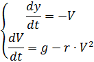
This problem can be solved with the help of a system of two differential equations, which are given below (excluding parachutes and changes in air density):

The change in resistance and air density is given in the listing under the spoiler, taking into account the above, and without explanation.

# - * - coding: utf8 - * -
from numpy import *
from scipy.integrate import odeint
import matplotlib.pyplot as plt
m = 100
r0 = 1.3
c1 = 0.3
c2 = 0.6
c3 = 0.5
c4 = 0.75
S = 70
s = 0.8
ss = 1.5
g = 9.8
tsp = 6
tsbp = 10
tp = 90.0
h = 1000.0
beta = 1.25 * 10 ** - 4
alfa = 6.5 * 10 ** - 3
T0 = 300
def ks (t):
if t <tsp:
z = 0
else:
z = 1
return z
def ko (t):
if t <tsp + tsbp:
z = 0
else:
z = 1
return z
# dy1 / dt = y2
# dy2 / dt = g- (k1 * y2 ** 2) / m- (k2 * y2) / m- (ks (t) * k3 * y2 ** 2) / m- (ko (t) * k4 * y2 ** 2) / m
def f (y, t):
y1, y2 = y
r = r0 * exp (-beta * y1 * T0 / (T0-alfa * y1))
k1 = 0.5 * r * c1 * s
k2 = 0.5 * r * c2 * s
k3 = 0.5 * r * c3 * ss
k4 = 0.5 * r * c4 * S
return [-y2, g- (k1 * y2 ** 2) / m- (k2 * y2) / m- (ks (t) * k3 * y2 ** 2) / m- (ko (t) * k4 * y2 ** 2) / m]
t = arange (0.0, tp)
y0 = [h, 0.0]
[y1, y2] = odeint (f, y0, t, full_output = False) .T
plt.title (“Skydiving from 1000 and 800 meters”)
plt.plot (y1, y2, label = 'Height 1000 m')
h = 800.0
tsp = 6
tsbp = 2
tp = 80.0
def ks (t):
if t <tsp:
z = 0
else:
z = 1
return z
def ko (t):
if t <tsp + tsbp:
z = 0
else:
z = 1
return z
def f (y, t):
y1, y2 = y
r = r0 * exp (-beta * y1 * T0 / (T0-alfa * y1))
k1 = 0.5 * r * c1 * s
k2 = 0.5 * r * c2 * s
k3 = 0.5 * r * c3 * ss
k4 = 0.5 * r * c4 * S
return [-y2, g- (k1 * y2 ** 2) / m- (k2 * y2) / m- (ks (t) * k3 * y2 ** 2) / m- (ko (t) * k4 * y2 ** 2) / m]
t = arange (0.0, tp)
y0 = [h, 0.0]
[y1, y2] = odeint (f, y0, t, full_output = False) .T
plt.plot (y1, y2, label = 'Height 800 m')
plt.xlabel ('Height in m.')
plt.ylabel ('speed of burning in m / s.')
plt.legend (loc = 'best')
plt.grid (true)
plt.show ()

We get:

Conclusion

The ballistic-temporal characteristics of the motion of the center of mass of a parachutist, landed from an airplane, are determined.