"Research into the job market for analysts" sounded like the very real task of a very real leading analyst of one large or small company. The parser tester is dozens of job descriptions with hh manually, scattering them over the requested skills and increasing the counter in the corresponding spreadsheet.

I saw in this task a good field for automation and decided to try to cope with it with less blood, easily and simply.

I was interested in the following questions raised in this study:

• the average salary level of business and system analysts,
• the most popular skills and personal qualities in this position,
• dependencies (if any) between certain skills and the level of salaries.

Spoiler: easy and simple failed.

Data preparation

If we want to collect a lot of data about vacancies, then it’s logical for hh not to be limited. However, for purity experiment simplicity start with this resource.

Collection

To collect data, we use the search for vacancies through the hh API.

I will search using a simple text query "systems analyst", "business analyst" and "product owner", because the activities and areas of responsibility of these positions, as a rule, overlap.

To do this, create a request of the form https://api.hh.ru/vacancies?text="systems+analyst" and parse the resulting JSON.

In order to get the most relevant vacancies in the sample, we will search only in vacancy headers, adding the search_field=name parameter to the query.

Here you can see which job fields are returned by this request. I chose the following:

• job title
• city
• publication date
• salary - upper and lower bounds
• currency in which the salary is specified
• gross - T / F
• company
• duties
• Requirements for a candidate

In addition, I want to further analyze the skills that are listed in the "Key Skills" section, but this section is available only in the full description of the vacancy. Therefore, I will also save the links to the found jobs in order to subsequently get a list of skills for each of them.

 #     :) library(jsonlite) library(curl) library(dplyr) library(ggplot2) library(RColorBrewer) library(plotly) hh.getjobs <- function(query, paid = FALSE) { # Makes a call to hh API and gets the list of vacancies based on the given search queries df <- data.frame( query = character() #    , URL = character() #    , id = numeric() # id  , Name = character() #   , City = character() , Published = character() , Currency = character() , From = numeric() # .    , To = numeric() # .  , Gross = character() , Company = character() , Responsibility = character() , Requerement = character() , stringsAsFactors = FALSE ) for (q in query) { for (pageNum in 0:99) { try( { data <- fromJSON(paste0("https://api.hh.ru/vacancies?search_field=name&text=\"" , q , "\"&search_field=name" , "&only_with_salary=", paid ,"&page=" , pageNum)) df <- rbind(df, data.frame( q, data$items$url, as.numeric(data$items$id), data$items$name, data$items$area$name, data$items$published_at, data$items$salary$currency, data$items$salary$from, data$items$salary$to, data$items$salary$gross, data$items$employer$name, data$items$snippet$responsibility, data$items$snippet$requirement, stringsAsFactors = FALSE)) }) print(paste0("Downloading page:", pageNum + 1, "; query = \"", q, "\"")) } } names <- c("query", "URL", "id", "Name", "City", "Published", "Currency", "From", "To", "Gross", "Company", "Responsibility", "Requirement") colnames(df) <- names return(df) } 

In the hh.getjobs() function, the vector accepts the search queries that we are interested in and the refinement, we are interested only in vacancies with a specified salary or everything (we take the second option by default). An empty dafa frame is created, and then the fromJSON() package fromJSON() function is used, which accepts a URL as input and returns a structured list. Next, from the nodes of this list, we extract the data of interest to us and fill in the corresponding data frame fields.

By default, data is given page by page, with 20 elements on each page. A maximum of one request, you can get 2000 jobs. All the data we write in df .

Life hacking 1: it’s not at all the fact that there are 2000 vacancies at our request, and starting from a certain moment we will receive blank pages. In this case, R swears and jumps out of the loop. Therefore, we carefully wrap the contents of the inner loop in try() .

Layfkhak 2: it also makes sense to add the output to the console of the current status of data collection, because this is not a quick matter. I did this:

 print(paste0("Downloading page:", pageNum + 1, "; query = \"", query, "\"")) 

After the data is filled, the columns are renamed so that it is convenient to work with them, and the resulting data frame is returned.

I will store this and other auxiliary functions in a separate functions.R file so as not to clutter up the main script, which so far looks like this:

 source("functions.R") # Step 1 - get data # 1.1 get vacancies (short info) jobdf <- hh.getjobs(query = c("business+analyst" , "systems+analyst" , "product+owner"), paid = FALSE) 

Now from the full description of vacancies we will get out the experience and key_skills .

The functions hh.getxp are hh.getxp data frame, we pass through the saved references to vacancies, and from the full description we get the value of the required work experience. The resulting value is stored in the new column.

 hh.getxp <- function(df) { df$experience <- NA for (myURL in df$URL) { try( { data <- fromJSON(myURL) df[df$URL == myURL, "experience"] <- data$experience$name } ) print(paste0("Filling in ", which(df$URL == myURL, arr.ind = TRUE), "from ", nrow(df))) } return(df) } 

The description of the new auxiliary function is sent to functions.R , and the main script now refers to it:

 # s.1.2 get experience (from full info) jobdf <- hh.getxp(jobdf) # 1.3 get skills (from full info) all.skills <- hh.getskills(jobdf$URL) 

In the fragment above, we also all.skills a new data frame all.skills form "vacancy id - skill":

 hh.getskills <- function(allurls) { analyst.skills <- data.frame( id = character(), # id  skill = character() #   ) for (myURL in allurls) { data <- fromJSON(myURL) if (length(data$key_skills) > 0) analyst.skills <- rbind(analyst.skills, cbind(data$id, data$key_skills)) print(paste0("Filling in " , which(allurls == myURL, arr.ind = TRUE) , " out of " , length(allurls))) } names(analyst.skills) <- c("id", "skill") analyst.skills$skill <- tolower(analyst.skills$skill) return(analyst.skills) } 

Preprocessing

Let's see how much data we managed to collect:

 > length(unique(jobdf$id)) [1] 1478 > length(jobdf$id) [1] 1498 

Almost one and a half thousand vacancies! Looks good. And apparently, several vacancies were caught in the search results twice - for different queries. Therefore, first of all, we will leave only unique entries: jobdf <- jobdf[unique(jobdf$id),] .

In order to compare the salaries of analysts on the labor market, I need

1) make sure that all available data on salaries are presented in a single currency,

2) highlight in a separate data frame those vacancies for which the salary is specified.

Consider each of the subtasks in more detail. Previously, you can find out which, in principle, currencies are found in our data using the table(jobdf$Currency) . In my case, in addition to rubles, there were dollars, euros, hryvnias, Kazakh tenges, and even Uzbek soums.

To convert salary values ​​to ruble, you need to know the current exchange rate. We will learn from the Central Bank :

 quotations.update <- function(currencies) { # Parses the most up-to-date qutations data provided by the Central Bank of Russia # and returns a table with currency rate against RUR doc <- XML::xmlParse("http://www.cbr.ru/scripts/XML_daily.asp") quotationsdf <- XML::xmlToDataFrame(doc, stringsAsFactors = FALSE) quotationsdf <- select(quotationsdf, -Name) quotationsdf$NumCode <- as.numeric(quotationsdf$NumCode) quotationsdf$Nominal <- as.numeric(quotationsdf$Nominal) quotationsdf$Value <- as.numeric(sub(",", ".", quotationsdf$Value)) quotationsdf$Value <- quotationsdf$Value / quotationsdf$Nominal quotationsdf <- quotationsdf %>% select(CharCode, Value) return(quotationsdf) } 

For courses to be processed correctly in R, you need to make sure that the decimal part is separated by a dot. In addition, you should pay attention to the Nominal column: somewhere it is 1, somewhere 10 or 100. This means one pound sterling costs ~ 85 rubles, and, say, for a hundred Armenian drams you can buy ~ 13 rubles. For the convenience of further processing, I brought the values ​​to par 1 against the ruble.

Now you can translate. Our script does this using the convert.currency() function. The current exchange rate in it is taken from the quotations table, where we have saved the data from the XML provided by the Central Bank. Also, at the input, the function accepts the target currency for conversion (by default RUR) and a table with vacancies, the salary forks values ​​in which must be converted to a single currency. The function returns a table with updated salary digits (already without the Currency column, as unnecessary).

I had to tinker with Belarusian rubles: after receiving very strange data in several approaches, I did a little research and found out that since 2016 Belarus has been using a new currency, which differs not only in exchange rate, but also in abbreviation (now not BYR, but BYN) . The hh reference books still use the BYR abbreviation, about which the XML from the Central Bank knows nothing. Therefore, in the convert.currency() function, I not the most elegant way I first replace the abbreviation with the current one, and only then I turn directly to the conversion.

It all looks like this:

 convert.currency <- function(targetCurrency = "RUR", df, quotationsdf) { cond <- (!is.na(df$Currency) & df$Currency == "BYR") df[cond, "Currency"] <- "BYN" currencies <- unique(na.omit(df$Currency[df$Currency != targetCurrency])) #     ( ) if (!is.null(df$From)) { for (currency in currencies) { condition <- (!is.na(df$From) & df$Currency == currency) try( df$From[condition] <- df$From[condition] * quotationsdf$Value[quotationsdf$CharCode == currency] ) } } #     ( ) if (!is.null(df$To)) { for (currency in currencies) { condition <- !is.na(df$To) & df$Currency == currency try( df$To[condition] <- df$To[condition] * quotationsdf$Value[quotationsdf$CharCode == currency] ) } } return(df %>% select(-Currency)) } 

It is also possible to take into account that some data on salaries are presented in gross values, that is, an employee will receive slightly less money. To calculate the net salary for residents of the Russian Federation, it is necessary to subtract 13% from the indicated figures (30% is deducted for non-residents).

 gross.to.net <- function(df, resident = TRUE) { if (resident == TRUE) coef <- 0.87 else coef <- 0.7 if (!is.null(df$Gross)) { if (!is.null(df$From)) #     ( ) { index <- na.omit(as.numeric(rownames(df[!is.na(df$From) & df$Gross == TRUE,]))) df$From[index] <- df$From[index] * coef } if (!is.null(df$To)) #     ( ) { index <- na.omit(as.numeric(rownames(df[!is.na(df$To) & df$Gross == TRUE,]))) df$To[index] <- df$To[index] * coef } df <- df %>% select(-Gross) } return(df) } 

Of course, I will not do this, because in this case it is necessary to take into account taxes in different countries, not only in Russia, or add a filter by country to the initial search query.

The last step before the analysis is to divide the vacancies into three categories: June, Middles and Seniors, and write the resulting positions in a new column. For senior positions we will include those with the word "senior" in their names and its synonyms. Similarly, we will find the starting positions for the keywords "junior" and synonyms, and we’ll take all those who are between:

 get.positions <- function(df) { df$lvl <- NA df[grep(pattern = "lead|senior|||", x = df$Name, ignore.case = TRUE), "lvl"] <- "senior" df[grep(pattern = "junior|||", x = df$Name, ignore.case = TRUE), "lvl"] <- "junior" df[is.na(df$lvl), "lvl"] <- "middle" return(df) } 

Add the data preparation block to the main script.

 # Step 2 - prepare data # 2.1. Convert all currencies to target currency # 2.1.1 get up-to-date currency rates quotations <- quotations.update() # 2.1.2 convert to RUR jobdf <- convert.currency(df = jobdf, quotationsdf = quotations) # 2.2 convert Gross to Net # jobdf <- gross.to.net(df = jobdf) # 2.3 define segments jobdf <- get.positions(jobdf) 

Analysis

As mentioned above, I am going to analyze the following aspects of the data obtained:

• average salary level BA / SA,
• the most popular skills and personal qualities in this position,
• dependencies (if any) between certain skills and the level of salaries.

Average income BA / SA

As it turned out, companies are reluctant to indicate the upper or lower salary limit.

In our data frame jobdf these values ​​are in the To and From columns, respectively. I want to find the average values ​​and write them to the new Salary column.

For cases where the salary is specified in full, this can be easily done using the mean() function, filtering out all other records where the data on the fork is missing completely or partially. But in this case, our initial sample, which is already small, would have remained less than 10%. Therefore, I calculate the coefficient Podgoniana which suggests how much the To and From values ​​differ on average in vacancies where the full fork is indicated, and with its help approximately fill in the missing data in cases where only one value is missing.

 select.paid <- function(df, suggest = TRUE) { # Returns a data frame with average salaries between To and From # optionally, can suggest To or From value in case only one is specified if (suggest == TRUE) { df <- df %>% filter(!is.na(From) | !is.na(To)) magic.coefficient <- # shows the average difference between max and min salary round(mean(df$To/df$From, na.rm = TRUE), 1) df[is.na(df$To),]$To <- df[is.na(df$To),]$From * magic.coefficient df[is.na(df$From),]$From <- df[is.na(df$From),]$To / magic.coefficient } else { df <- na.omit(df) } df$salary <- rowMeans(x = df %>% select(From, To)) df$salary <- ceiling(df$salary / 10000) * 10000 return(df %>% select(-From, -To)) } 

This is a “soft” data filtering, which in the select.paid() function is set by the parameter suggest = TRUE . Alternatively, we can specify suggest = FALSE when calling a function and simply cut out all the lines where salary data is at least partially missing. However, using soft filtering and a magic coefficient, I managed to save almost a quarter of the original data set in the sample.

Go to the visual part:

On this graph, you can visually assess the distribution density of salaries BA / SA in the two capitals and in the regions. But what if to specify a request and compare how much middles and seniors receive in capitals?

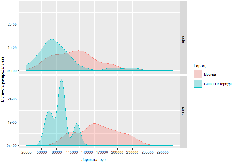
From the resulting schedule it is clear that the difference in salary situations for middles and seniors in Moscow and St. Petersburg is not too different. For example, in St. Petersburg, midls are usually obtained in the region of 70 TR, while in Moscow the density peak is ~ 120 TR, and the difference in incomes of senior level specialists in Moscow and St. Petersburg differs by an average of 60 thousand.

We can also look, for example, at Moscow analyst salaries in the context of the post:

It can be concluded that a) today there is much greater demand for entry-level analyst analysts in Moscow, and b) at the same time, the upper salary threshold of such specialists is limited much more clearly than among middles and seniors.

Another observation: the average sn Moscow mid-level and high-level specialists have a rather large intersection area. This may indicate that the market has a rather blurred border between these two steps.

Full code for graphs under the cut.

 # Step 3 - analyze salaries # 3.1 get paid jobs (with salaries specified) jobs.paid <- select.paid(jobdf) # 3.2 plot salaries density by region ggplotly(ggplot(jobs.paid, aes(salary, fill = region, colour = region)) + geom_density(alpha=.3) + scale_fill_discrete(guide = guide_legend(reverse=FALSE)) + scale_x_continuous(labels = function(x) format(x, scientific = FALSE), name = ", .", breaks = round(seq(min(jobs.paid$salary), max(jobs.paid$salary), by = 30000),1)) + scale_y_continuous(name = " ") + theme(axis.text.x = element_text(size=9), axis.title = element_text(size=10))) # 3.3 compare salaries for middle / senior in capitals ggplot(jobs.paid %>% filter(region %in% c("", "-"), lvl %in% c("senior", "middle")), aes(salary, fill = region, colour = region)) + facet_grid(lvl ~ .) + geom_density(alpha = .3) + scale_x_continuous(labels = function(x) format(x, scientific = FALSE), name = ", .", breaks = round(seq(min(jobs.paid$salary), max(jobs.paid$salary), by = 30000),1)) + scale_y_continuous(name = " ") + scale_fill_discrete(name = "") + scale_color_discrete(name = "") + guides(fill=guide_legend( keywidth=0.1, keyheight=0.1, default.unit="inch") ) + theme(legend.spacing = unit(1,"inch"), axis.title = element_text(size=10)) # 3.4 plot salaries in Moscow by position ggplotly(ggplot(jobs.paid %>% filter(region == ""), aes(salary, fill = lvl, color = lvl)) + geom_density(alpha=.4) + scale_fill_brewer(palette = "Set2") + scale_color_brewer(palette = "Set2") + theme_light() + scale_y_continuous(name = " ") + scale_x_continuous(labels = function(x) format(x, scientific = FALSE), name = ", .", breaks = round(seq(min(jobs.paid$salary), max(jobs.paid$salary), by = 30000),1)) + theme(axis.text.x = element_text(size=9), axis.title = element_text(size=10))) 

Analysis of skills (Key skills)

Moving on to the key goal of the study is to identify the most relevant skills for BA / SA. To do this, we will analyze those data that are explicitly indicated in a special vacancy field - key skills.

Most popular skills

Previously, we received a separate data frame all.skills , where we recorded pairs of "vacancy id - skill". Finding the most common skills is easy with the table() function:

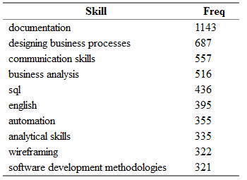
 tmp <- as.data.frame(table(all.skills$skill), col.names = c("Skill", "Freq")) htmlTable::htmlTable(x = head(tmp[order(tmp$Freq, na.last = TRUE, decreasing = TRUE),]), rnames = FALSE, header = c("Skill", "Freq"), align = 'l', css.cell = "padding-left: .5em; padding-right: 2em;") 

It turns out about the following:

Here Freq is the number of vacancies, in the "key_skills" field of which the corresponding skill is indicated from the Skill column.

“But that's not all!” (C) It is quite obvious that the same skills can easily be found in different vacancies in synonymous expressions.

I have compiled a small dictionary of synonyms for the names of skills and divided them into categories.

A dictionary is a csv file with category columns — one of the following: Activities, Tools, Knowledge, Standards, and Personal; skill - the main name of the skill, which I will use instead of all the synonyms found; syn1, syn2, ... syn13 - actually possible variations for each skill. Some lines may contain empty synonym columns.

 category;skill;syn1;syn2;syn3;syn4;syn5;syn6;syn7;syn8;syn9;syn10;syn11;syn12;syn13 tools;axure;;;;;;;;;;;;; tools;lucidchart;;;;;;;;;;;;; standards;archimate;;;;;;;;;;;;; standards;uml;activity diagram;use case diagram;ucd;class diagram;;;;;;;;; personal;teamwork;team player;  ;;;;;;;;;;; activities;wireframing;mockup;mock-up;;-;wireframe;;ui;ux/;/ux;;;; 

We first import the dictionary, and then scatter skills again based on the existing equivalences:

 # Analyze skills # 4.1 import dictionary dict <- read.csv(file = "competencies.csv", header = TRUE, stringsAsFactors = FALSE, sep = ";", na.strings = "", encoding = "UTF-8") # 4.2 match skills with dictionary all.skills <- categorize.skills(all.skills, dict) 

Under the cut, you can see the filling of the function categorize.skills() .

 categorize.skills <- function(analyst_skills, dictionary) { analyst_skills$skill.group <- NA analyst_skills$category <- NA for (myskill in dictionary$skill) { category <- dictionary[dictionary$skill == myskill, "category"] mypattern <- paste0(na.omit(t(dictionary %>% filter(skill == myskill) %>% select(starts_with("syn")))), collapse = "|") if (nchar(mypattern) > 1) mypattern <- paste0(c(myskill, mypattern), collapse = "|") else mypattern <- myskill try( { analyst_skills[grep(x = analyst_skills$skill, pattern = mypattern),"skill.group"] <- myskill analyst_skills[grep(x = analyst_skills$skill, pattern = mypattern),"category"] <- category } ) } return(analyst_skills) } 

I add the category column and the column to the initial data frame with skills. group - for the category and the generic name of the skill, respectively. Then I go through the imported dictionary and from each line of synonyms make a pattern for the grep() function. By adding each non-empty column value to a line, I separate them with a dash to get the condition "or". So, for all skills from the source table that include the uml|activity diagram|use case diagram|ucd|class diagram , I’ll write the value "uml" in the skill.group column. And so it will be with everyone! .. skill from the original data frame.

Re-requesting the top most popular skills, you can see that the alignment of forces has changed somewhat:

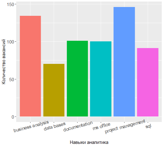
The top three are project management, business analysis and documentation, and knowledge of UML has shifted from the top 7.

Quite interesting to go through the categories and find out what skills are most in demand in each of them.

For example, for the Knowledge category, the situation is as follows:

 tmp <- merge(x = all.skills, y = jobdf %>% select(id, lvl), by = "id", sort = FALSE) tmp <- na.omit(tmp) ggplot(as.data.frame(table(tmp %>% filter(category == "knowledge") %>% select(skill.group)))) + geom_bar(colour = "#666666", stat = "identity", aes(x = reorder(Var1, Freq), y = Freq, fill = reorder(Var1, -Freq))) + scale_y_continuous(name = " ") + theme(legend.position = "none", axis.text = element_text(size = 12)) + coord_flip() 

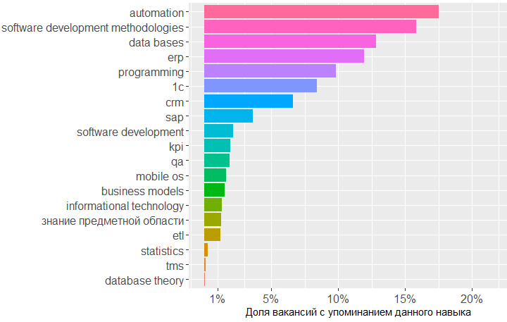
From the graph it is seen that knowledge in the field of databases, software development methodologies and 1C are in greatest demand. Next comes knowledge of CRM, ERP systems and the basics of programming.

As far as standards are concerned, knowledge of SQL and UML is really in demand, ARIS notation comes on its heels, but GOSTs take only the sixth place.

 ggplot(as.data.frame(table(tmp %>% filter(category == "standards") %>% select(skill.group)))) + geom_bar(colour = "#666666", stat = "identity", aes(x = reorder(Var1, Freq), y = Freq, fill = Var1)) + scale_y_continuous(name = " ") + theme(legend.position = "none", axis.text = element_text(size = 12)) + coord_flip() 

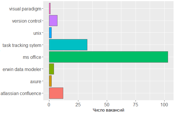
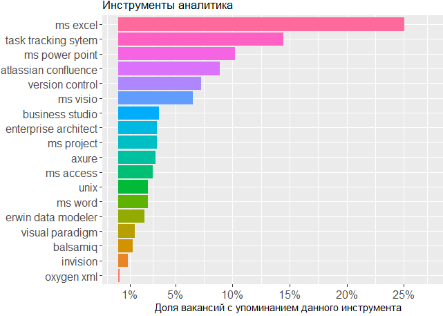
As for the bodies used, we once again confirm that the main tool of the analyst is the head. Without a line of MS Office and task-tracking systems is not enough, but for the rest, few people care about which editor the analyst creates his schemes or throws interface layouts.

 ggplot(tmp %>% filter(category == "tools")) + geom_histogram(colour = "#666666", stat = "count", aes(skill.group, fill = skill.group)) + scale_y_continuous(name = " ") + theme(legend.position = "none", axis.text = element_text(size = 12)) + coord_flip() 

Impact of skills on income

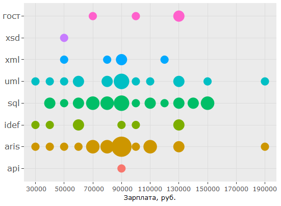
Finally, let us analyze the range of salaries for references to various skills. , , , .

jobs.paid all.skills , data frame.

 # 4.4 vizualize paid skills tmp <- na.omit(merge(x = all.skills, y = jobs.paid %>% select(id, salary, lvl, City), by = "id", sort = FALSE)) 

:

 > head(tmp) id skill skill.group category salary lvl City 2 25781585 android mobile os knowledge 90000 middle  3 25781585   project management activities 90000 middle  5 25781585   project management activities 90000 middle  6 25781585 ios mobile os knowledge 90000 middle  7 25750025 aris aris standards 70000 middle  8 25750025 - business analysis activities 70000 middle  

, .. . :

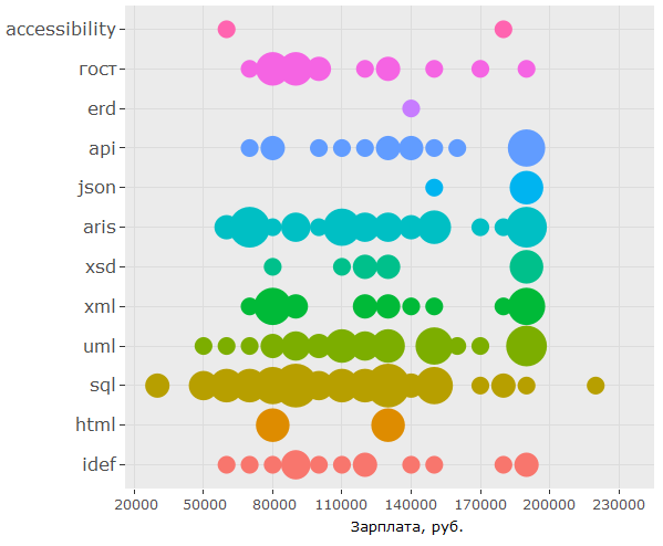
 ggplotly(ggplot(tmp %>% filter(category == "activities"), aes(skill.group, salary)) + coord_flip() + geom_count(aes(size = ..n.., color = City)) + scale_fill_discrete(name = "") + scale_y_continuous(name = ", .") + scale_size_area(max_size = 11) + theme(legend.position = "bottom", axis.title = element_blank(), axis.text.y = element_text(size=10, angle=10))) 

, BA/SA .

:

 ggplot(tmp %>% filter(category == "personal", City %in% c("", "-")), aes(tools::toTitleCase(skill), salary)) + coord_flip() + geom_count(aes(size = ..n.., color = skill.group)) + scale_y_continuous(breaks = round(seq(min(tmp$salary), max(tmp$salary), by = 20000),1), name = ", .") + scale_size_area(max_size = 10) + theme(legend.position = "none", axis.title = element_text(size = 11), axis.text.y = element_text(size=10, angle=0)) 

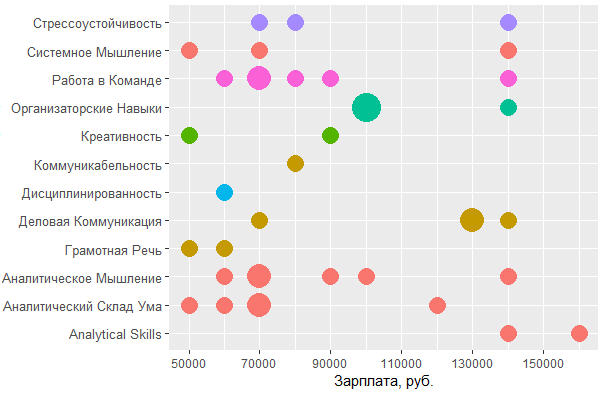
, MS Office , — , - . , , , .

, , : UML ARIS, SQL ( ) , IDEF — , "".

, , , . , 1478 - key_skills. , - .

, data frame:

 > jobdf$Responsibility[[1]] [1] "Training course in business analysis. ● Define needs of the user/client, understand the problem which needs to be solved. ● " > jobdf$Requirement[[1]] [1] "At least 6 months' experience in business analysis. ● Knowledge of qualitative methods such as usability testing, interviewing, focus groups. ● " 

, , . URL' , .

 hh.get.full.desrtion <- function(df) { df$full.description <- NA for (myURL in df$URL) { try( { data <- fromJSON(myURL) if (length(data$description) > 0) { df$full.description[which(df$URL == myURL, arr.ind = TRUE)] <- data$description } print(paste0("Filling in " , which(df$URL == myURL, arr.ind = TRUE) , " out of " , length(df$URL))) } ) } df$full.description <- tolower(df$full.description) return(df) } 

- , html- ., gsub :

 remove.Html <- function(htmlString) { #remove html tags return(gsub("<.*?>", "", htmlString)) } 

, , , , . data frame ( df), , df "id, skill.group, category".

 skills.from.desc <- function(df, dictionary) { sk <- data.frame( id = numeric() , skill.group = character() , category = character() ) for (myskill in dictionary$skill) { category <- dictionary[dictionary$skill == myskill, "category"] mypattern <- paste0(na.omit(t(dictionary %>% filter(skill == myskill) %>% select(starts_with("syn")))), collapse = "|") if (nchar(mypattern) > 1) { mypattern <- paste0(c(myskill, mypattern), collapse = "|") } else { mypattern <- myskill } cond = grep(x = df$full.description, pattern = mypattern) tmp <- data.frame( id = df[cond, "id"], skill.group = rep(myskill, length(cond)), category = rep(category, length(cond)) ) sk <- rbind(sk, tmp) } return(sk) } 

 # 5 text analysis # 5.1 get full descriptions jobdf <- hh.get.full.description(jobdf) jobdf$full.description <- remove.Html(tolower(jobdf$full.description)) sk.from.desc <- skills.from.desc(jobdf, dict) 

, ?

 > head(sk.from.desc) id skill.group category 1 25638419 axure tools 2 24761526 axure tools 3 25634145 axure tools 4 24451152 axure tools 5 25630612 axure tools 6 24985548 axure tools > tmp <- as.data.frame(table(sk.from.desc$skill.group), col.names = c("Skill", "Freq")) > htmlTable::htmlTable(x = head(tmp[order(tmp$Freq, na.last = TRUE, decreasing = TRUE),], 20), rnames = FALSE, header = c("Skill", "Freq"), align = 'l', css.cell = "padding-left: .5em; padding-right: 2em;") 

, ! Project management, key_skills, ( ).

, , key_skills -5.

, . 1478 , , key_skills, , .

, , BA , - .

, .

data frame , , . , -.

 tmp <- na.omit(merge(x = sk.from.desc, y = jobs.paid %>% filter(City %in% c("", "-")) %>% select(id, salary, lvl, City), by = "id", sort = FALSE)) 

 > head(tmp) id skill.group category salary lvl City 1 25243346 uml standards 160000 middle  2 25243346 requirements management activities 160000 middle  3 25243346 designing business processes activities 160000 middle  4 25243346 communication skills personal 160000 middle  5 25243346 mobile os knowledge 160000 middle  6 25243346 ms visio tools 160000 middle  

, , , .

 ggplotly(ggplot(tmp %>% filter(category == "activities"), aes(skill.group, lvl)) + geom_count(aes(color = salary, size = ..n..)) + scale_size_area(max_size = 13) + theme(legend.position = "right", legend.title = element_text(size = 10), axis.title = element_blank(), axis.text.y = element_text(size=10)) + coord_flip() + scale_color_continuous(labels = function(x) format(x, scientific = FALSE), breaks = round(seq(min(tmp$salary), max(tmp$salary), by = 70000),1), low = "blue", high = "red", name = ", .")) 

?

-, , - . ( , , , .)

-, , "" -, .

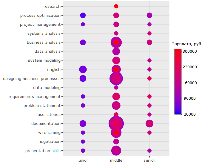
, key_skills.

, , 150 .. UML ARIS, IDEF, , — .

:

, - , , key_skills , . , 150 .. , .

?

, - :

, , , ? , . , , . , ó ( ) .

, - :

-

BA/SA ,

• . , ;
• ( ) 200 .. , , ;
• ;
• — - ( , , )
• key_skills hh , ;
• , , , (!) ;
• , -, UX ;
• . , - 150 ..;
• , , SQL, UML & ARIS. , .. . , , , .

 wordcloud2::wordcloud2(data = table(sk.from.desc$skill.group), rotateRatio = 0.3, color = 'random-dark')