Determination of gas density from the results of measuring pressure and temperature with Arduino sensors

Introduction

The task of measuring the parameters of a gas mixture is widespread in industry and commerce. The problem of obtaining reliable information when measuring the parameters of the state of the gas environment and its characteristics with the help of technical means is resolved by standard measurement techniques (MVI), for example, when measuring the flow and amount of gases using standard narrowing devices [1], or using turbine, rotary and vortex flowmeters and counters [2].

Periodic gas analysis allows to establish the correspondence between the actual mixture being analyzed and its model, according to which the physicochemical parameters of the gas are taken into account in the MVI: the composition of the gas mixture and the density of the gas under standard conditions.
MVI also takes into account the thermophysical characteristics of the gas: the density at the operating conditions (pressure and temperature of the gas at which measurement of its flow or volume is performed), viscosity, factor and compressibility factor.

The parameters of gas state measured in real time include pressure (pressure differential), temperature, density. Means of measuring equipment are used to measure these parameters: manometers (differential pressure gauges), thermometers, and density meters. Measurement of the density of the gas medium can be measured directly or indirectly by measurement methods. The results of both direct and indirect measurement methods depend on the error of the measuring instrument and the methodical error. Under operating conditions, the measurement information signals may be subject to significant noise, the standard deviation of which may exceed the instrumental error. In this case, the actual task is the effective filtering of measurement information signals.

This article discusses the method of indirect measurement of gas density under operating and standard conditions using the Kalman filter.

Mathematical model for determining gas density

Let us turn to the classics and recall the equation of state of an ideal gas [3]. We have:

1. The Mendeleev-Clapeyron equation:

(one),

Where:

- gas pressure;

- molar volume;

R is the universal gas constant,

;

T is the absolute temperature, T = 273.16 K.

2. Two measured parameters:

p - gas pressure, Pa
t is the gas temperature, ° .

It is known that the molar volume depends on the volume of gas V and the number of moles of gas in this volume:

(2)

It is also known that

(3)

where: m is the mass of a gas, M is the molar mass of a gas.

Given (2) and (3), we rewrite (1) in the form:

(four).

As is known, the density of matter

equals:

(five).

From (4) and (5) we derive the equation for the gas density

:

(6)

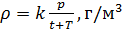
and enter the parameter designation

which depends on the molar mass of the gas mixture:

(7).

If the composition of the gas mixture does not change, then the parameter k is constant.
So, to calculate the gas density, it is necessary to calculate the molar mass of the gas mixture.

The molar mass of the mixture of substances is determined as the arithmetic average weighted molar mass of the mass fractions included in the mixture of individual substances.

We take the known composition of substances in the gas mixture - in the air, which consists of:

• 23% by weight of oxygen molecules
• 76% by weight of nitrogen molecules
• 1% by weight of argon atoms

The molar masses of these air substances will be respectively equal to:

g / mol.

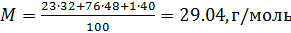
Calculate the molar mass of air, as the weighted average:



Now, knowing the value of a constant

, we can calculate the air density by the formula (7) taking into account the measured values

and t :

Reducing gas density to normal, standard conditions

In practice, measurements of the properties of gases are carried out in different physical conditions, and standard sets of conditions should be established to provide a comparison between different data sets [4].

Standard conditions for temperature and pressure are the physical conditions established by the standard to which properties of substances are correlated, depending on these conditions.

Various organizations set their standard conditions, for example: the International Union of Pure and Applied Chemistry (IUPAC), established the definition of standard temperature and pressure (STP) in the field of chemistry: temperature 0 ° C (273.15 K), absolute pressure 1 bar (Pa); The National Institute of Standards and Technology (NIST) sets a temperature of 20 ° C (293.15 K) and an absolute pressure of 1 atm (101.325 kPa), and this standard is called the normal temperature and pressure (NTP); The International Organization for Standardization (ISO) establishes standard conditions for natural gas (ISO 13443: 1996, confirmed in 2013): a temperature of 15.00 ° C and an absolute pressure of 101.325 kPa.

Therefore, in industry and commerce it is necessary to specify the standard conditions for temperature and pressure, relative to which and to carry out the necessary calculations.

We calculate the air density by equation (8) under the working conditions of temperature and pressure. In accordance with (6), we write the equation for air density under standard conditions: temperature and absolute pressure :

(9).

We calculate the air density, reduced to standard conditions. We divide equation (9) into equation (6) and write this ratio for :

(ten).

In a similar way, we obtain the equation for calculating the density of air, reduced to normal conditions: temperature and absolute pressure

:

(eleven).

In equations (10) and (11) we use the values ​​of air parameters , T and P from equation (8), obtained under operating conditions.

The implementation of the measuring channel pressure and temperature

To solve many problems of obtaining information, depending on their complexity, it is convenient to create a prototype of a future system based on one of the microcontroller platforms such as Arduino, Nucleo, Teensy, and others.

What could be easier? Let's make a microcontroller platform for solving a specific task - creating a system for measuring pressure and temperature, spending less, possibly, means, and using all the advantages of developing software in the Arduino Software (IDE) environment.

For this, at the hardware level, we need the components:

1. Arduino (Uno, ...) - use as a programmer;
2. ATmega328P-PU microcontroller - a microcontroller of the future platform;
3. a 16 MHz crystal oscillator and a pair of ceramic capacitors of 12-22 pF each (as recommended by the manufacturer);
4. clock button to reset the microcontroller and pull-up plus power to the RESET pin of the microcontroller 1 kΩ resistor;
5. BMP180 - temperature and pressure measuring transducer with I2C interface;
6. TTL / USB interface converter;
7. consumables - wires, solder, circuit board, etc.

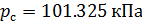
A schematic diagram of the platform, taking into account the necessary interfaces: standard serial interface, I2C, and nothing more, is presented in Fig. one.


Fig. 1 - Schematic diagram of the microcontroller platform for the implementation of a system for measuring pressure and temperature

Now consider the stages of our task.

1. First, we need a programmer. We connect Arduino (Uno, ...) to the computer. In the Arduno Software environment, from the menu along File-> Examples-> 11. ArdunoISP get to the programmer programmer ArduinoISP, which we sew in Arduino. Previously, from the Tools menu, select, respectively, the board, processor, bootloader, port. After loading the ArduinoISP program into the board, our Arduino turns into a programmer and is ready for use as intended. To do this, in the Arduno Software environment, in the Tools menu, select the Programmer item : “Arduino as ISP ”.

2. We connect via the SPI interface the slave microcontroller ATmega328P to the Arduino master programmer (Uno, ...), fig. 2. It should be noted that the pre-bits of the ATmega328P microcontroller's Low Fuse Byte register were set to the unprogrammed state. Go to the Arduno Software environment and from the Tools menu, select the Write Loader item. We are flashing the ATmega328P microcontroller.


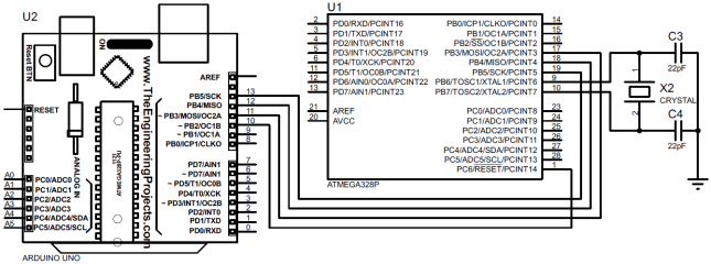Fig. 2 - Wiring diagram of the microcontroller to the programmer

3. After successful firmware, the ATmega328P microcontroller is ready for installation on the developed microcontroller platform (Fig. 3), which we program as well as the full Arduino (Uno, ...). A survey program for a pressure and temperature transmitter is shown in Listing 1.


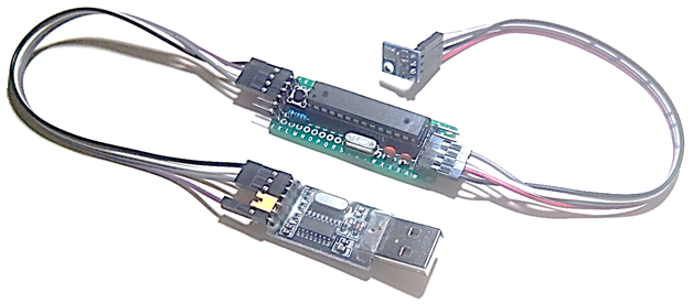Fig. 3 Pressure and temperature measurement system

Python program for filtering by temperature and pressure channels, and getting results

The Python program for determining gas density from pressure and temperature measurements is shown in Listing 2. Information from the measurement system is displayed in real time.


The calculation results are presented in listing and fig. 4, 5, 6.



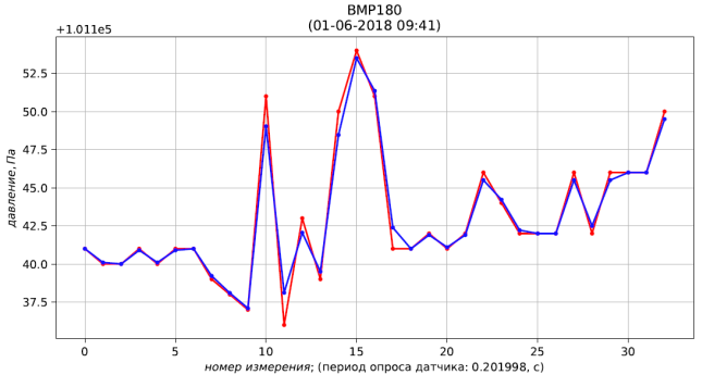Fig. 4 - measurement results (red) and filtration (blue) pressure


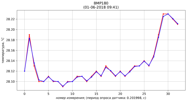Fig. 5 - measurement results (red) and filtration (blue) temperature


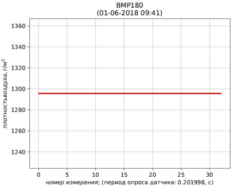Fig. 6 - results of calculation of air density, reduced to standard conditions (temperature 273.15 K; absolute pressure 101.325 kPa)

findings

A method has been developed for determining the density of a gas from the results of pressure and temperature measurements using Arduino sensors and Python software.

References to sources of information

1. GOST 8.586.5-2005. URL
2. GOST R 8.740 - 2011. URL
3. Ideal gas law. URL
4. Standard conditions for temperature and pressure. URL