
In our blog on Habré we published adapted translations of materials from The Financial Hacker blog, devoted to the issues of creating strategies for trading on the stock exchange. Earlier we discussed the
search for market inefficiencies , the creation of
models of trading strategies , and the
principles of their programming . Today we
will discuss the use of machine learning approaches to improve the efficiency of trading systems.
The first computer to win the World Chess Championship was Deep Blue. This was in 1996, and another twenty years passed before another program, Alpha Go, managed to defeat the best player in Go. Deep Blue was a model-oriented system with the rules of the game of chess. AplhaGo is a data-mining system, a deep neural network, trained with the help of thousands of games in Go. That is, in order to take a step from victories over people who are champions in chess, to dominate the top players in Go, it took not a improved piece of hardware, but a breakthrough in the field of software.
In the current article we will consider the application of the data mining approach to the creation of trading strategies. This method does not take into account market mechanisms; it simply scans price curves and other data sources to search for predictive patterns. Machine learning or “artificial intelligence” is not always necessary. On the contrary, very often, the most popular and profitable data mining methods work without any ryushechek in the form of neural networks or support for vector methods.
Principles of machine learning
The algorithm being taught is “fed” with data samples, usually somehow separated from historical stock prices. Each sample consists of n variables x1 ... xn, commonly referred to as predictors, functions, signals, or, more simply, input data. These predictors can be the prices of the last n bars on the price chart or a set of values of classical indicators, and any other functions of the price curve (there are even cases when individual pixels of the price chart are used as predictors for the neural network!). Each sample also usually contains some target variable y, for example, the result of the next deal after analyzing the sample or the next price movement.
In literature, y is often called a label or a goal (objective). In the process of learning, the algorithm learns to predict the target y based on the predictors x1 ... xn. What the system “remembers” in the process is stored in a data structure called a model that is specific to a particular algorithm (it is important not to confuse this concept with a financial model or a model-oriented strategy). A machine learning model can be a function with prediction rules written using a C code generated by the learning process. Or it could be a set of connected neural network weights:
Training: x1 ... xn, y => model
Prediction: x1 ... xn, model => y
Predictors, functions or whatever you want to call them, should contain information sufficient to generate predictions about the value of target y with a certain accuracy. They must also meet two formal criteria. First, all predictor values should be in the same range, for example, -1 ... +1 (for most algorithms on R) or -100 ... +100 (for algorithms in the Zorro or TSSB scripting languages). So, before sending the data to the system, you need to normalize them. Secondly, the samples must be balanced, that is, evenly distributed over the values of the target variable. That is, you must have the same number of samples leading to a positive outcome, and losing sets. If these two requirements are not followed, then good results will fail.
Regression algorithms generate predictions of numerical values, such as magnitude or sign of the next price movement. Classification algorithms predict quantitative classes of samples, for example, whether they precede profit or loss of funds. Some algorithms, such as neural networks, decision trees, or support vector machines, can be run in both modes.
There are also algorithms that can learn how to select from class samples without the need for a target y. This is called uncontrolled learning, as opposed to supervised learning. Somewhere between these two methods, there is “reinforced learning”, in which the system is trained by running simulations with specified functions and uses the result as a goal. A follower of AlphaGo, a system called AlphaZero used reinforced learning, playing a million Go games with itself. In finance, however, such systems or products using unsupervised learning are extremely rare. 99% of systems use supervised learning.
What signals we would not use for predictors in finance, in most cases they will contain a lot of noise and little information, and in addition they will be non-stationary. So financial predictions are one of the most difficult tasks of machine learning. More complex algorithms here achieve better results. Choosing predictors is critical to success. They do not have to be many, as this leads to retraining and malfunctioning. Therefore, data mining strategies often use a preselected algorithm that allocates a small number of predictors from a wider pool. Such preliminary selection can be based on the correlation between the predictors, their significance, information richness, or simply the success / failure of the use of the test set. Practical experiments with the selection of targets can be found, for example, in the blog
Robot Wealth .
Below is a list of the most popular data mining methods used in finance.
1. Soup from indicators
Most trading systems are not based on financial models. Often, traders need only trading signals generated by certain technical indicators, which are filtered by other indicators in combination with additional technical indicators. When such a trader is asked about how such a hodgepodge of indicators can lead to some kind of profit, he usually answers something like: “Believe me, I am trading with my hands and everything works.”
And it is true. At least sometimes. Although most of these systems will not pass the
WFA test (and some are simply tested on historical data), a surprisingly large number of such systems eventually work and make a profit. The author of the Financial Hacker blog is engaged in developing custom-made trading systems, and tells the story of one of the clients who systematically experimented with technical indicators until he found a combination of them that works for certain types of assets. Such a method of trial and error is a classic approach to data mining, for success you only need it, good luck and a lot of money for tests. As a result, you can sometimes expect to receive a profitable system.
2. Candle patterns
Not to be confused with the patterns of Japanese candles, which have existed for hundreds of years. The modern equivalent of this approach is trading based on price movements. You also analyze the open, high, low and close figures for each candle in the chart. But now you are using data mining to analyze the candles of the price curve to highlight patterns that can be used to generate predictions about the direction of price movement in the future.
There are entire software packages for this purpose. They look for patterns that are profitable in terms of user-defined criteria, and use them to build a pattern detection function. It all looks something like this:
int detect(double* sig) { if(sig[1]<sig[2] && sig[4]<sig[0] && sig[0]<sig[5] && sig[5]<sig[3] && sig[10]<sig[11] && sig[11]<sig[7] && sig[7]<sig[8] && sig[8]<sig[9] && sig[9]<sig[6]) return 1; if(sig[4]<sig[1] && sig[1]<sig[2] && sig[2]<sig[5] && sig[5]<sig[3] && sig[3]<sig[0] && sig[7]<sig[8] && sig[10]<sig[6] && sig[6]<sig[11] && sig[11]<sig[9]) return 1; if(sig[1]<sig[4] && eqF(sig[4]-sig[5]) && sig[5]<sig[2] && sig[2]<sig[3] && sig[3]<sig[0] && sig[10]<sig[7] && sig[8]<sig[6] && sig[6]<sig[11] && sig[11]<sig[9]) return 1; if(sig[1]<sig[4] && sig[4]<sig[5] && sig[5]<sig[2] && sig[2]<sig[0] && sig[0]<sig[3] && sig[7]<sig[8] && sig[10]<sig[11] && sig[11]<sig[9] && sig[9]<sig[6]) return 1; if(sig[1]<sig[2] && sig[4]<sig[5] && sig[5]<sig[3] && sig[3]<sig[0] && sig[10]<sig[7] && sig[7]<sig[8] && sig[8]<sig[6] && sig[6]<sig[11] && sig[11]<sig[9]) return 1; .... return 0; }
This C function returns 1 when the signal matches one of the patterns, otherwise it returns 0. A long code seems to hint that this is not the fastest way to find patterns. It is better to use an approach in which the detection function does not need to be exported, but can sort the signals by their importance and carry out the sorting. An example of such a system can be found
by reference .
Can “trade by price” work? As in the previous case, this method is not based on any rational financial model. At the same time, everyone understands that truly certain events in the market can influence its participants, as a result of which short-term predictive patterns arise. But the number of such patterns cannot be large if you study only a sequence of several consecutive candles on a chart. Then, it will be necessary to compare the result with the given candles, which are not near, but on the contrary, randomly selected on a longer time interval. In this case, you will get an almost unlimited number of patterns - and successfully break away from the concepts of reality and rationality. It is difficult to imagine how you can predict the future price, based on some of its values last week. Despite this, many traders are working in this direction.
3. Linear regression
A simple basis for a set of complex machine learning algorithms: predict the target variable y using a linear combination of predictors x1 ... xn.

Odds - this is the model. They are calculated to minimize the sum of standard deviations between the real values of y, the training values and the predicted y using the formula:
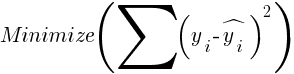
For normally distributed samples, minimization is possible using matrix operations, so no iteration is required. In the case when n = 1 - with only one predictor x, the regression formula is reduced to:

- that is, before simple linear regression, and when n> 1 linear regression will be multivariate. Simple linear regression is available in most trading platforms, for example,
LinReg indicator in TA-Lib. When y = price and x = time, it can be used as an alternative to a moving average. In the R platform, this regression is implemented by the standard delivery function lm (..). It can also be represented by polynomial regression. As in the simplest case, one predictive variable x is used here, but also its square and subsequent powers, so that xn == xn:
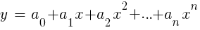
If n = 2 or n = 3, polynomial regression is often used to predict the next average price from the smoothed prices of the last bars. For polynomial regression, the polyfit function of MatLab, R, Zorro and many other platforms can be used.
4. Perceptron
Often it is called a neural network with only one neuron. In fact, the perceptron is a regression function, as described above, but with a binary result, as a result of which it is called a
logistic regression . Although in general it is not a regression, but a classification algorithm. For example, the advise function (PERCEPTRON, ...) of the Zorro framework generates C code that returns 100 or -100, depending on whether the predicted result is threshold or not:
int predict(double* sig) { if(-27.99*sig[0] + 1.24*sig[1] - 3.54*sig[2] > -21.50) return 100; else return -100; }
As it is easy to see, the sig array is equivalent to the functions xn in the regression formula, and the digital factors are the coefficients an.
5. Neural networks
Linear or logistic regression can solve only linear problems. At the same time, trading tasks often do not fit into this category. A famous example is the prediction of the output of a simple XOR function. This also includes the prediction of profit from transactions. An artificial neural network (ANN) can solve non-linear problems. This is a set of perceptrons that are connected to an array of different levels. Each perceptron is a neuron network. Its output becomes input for other neurons of the following level:
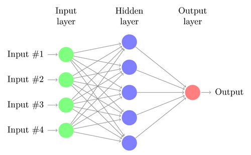
Like the perceptron, the neural network learns by determining coefficients that minimize the error between prediction and goal in the sample. This requires an approximation process, usually with back-propagation of the error from the output data to the input data with the associated optimization of weights. This process imposes two limitations. First, the output of neurons should be a continuously differentiated function instead of a simple threshold for the perceptron. Secondly, the network should not be very deep - the presence of a large number of hidden levels of neurons between the input and output data only harms. This second constraint limits the complexity of the problems that a standard neural network can solve.
When using neural networks to predict transactions, you will have many parameters with which you can manipulate, which, if done carelessly, can lead to the appearance of selection bias:
- the number of hidden levels;
- the number of neurons in each hidden level;
- the number of cycles of reverse propagation - epochs;
- degree of study, step width of the era;
- momentum, inertia factor to adapt weights;
- activation function.
The activation function emulates the threshold of the perceptron. For back propagation, a continuously differentiable function is needed that generates a soft step for a particular value of x. Usually, the functions sigmoid, tanh or softmax function are used for this. Sometimes a linear function is used that returns a weighted sum of all input data. In this case, the network can be used for regression, prediction of numerical values instead of binary output.
Neural networks are included in the standard package of R (for example, nnet is a network with one hidden level), as well as in many other packages (like RSNNS and FCNN4R).
6. Deep learning
In-depth training methods use neural networks with a large number of hidden levels and thousands of neurons that cannot be effectively trained using simple back propagation. In recent years, several methods have become popular for training such large networks. They usually imply prior learning of hidden levels of neurons to increase the effectiveness of basic learning.
The Restricted Boltzmann Machine (RBM) Restricted Machine is an uncontrolled classification algorithm with a special network structure that does not have connections between hidden neurons. The Sparse autocoder (SAE) uses a conventional network structure, but pre-trains hidden layers in a certain way, reproducing input signals to output levels with as few active connections as possible. These methods allow you to implement very complex networks for solving very complex learning problems. For example, the task of defeating the best man playing Go.
Deep learning networks are included in the deepnet and darch packages for R. The deepnet includes an auto-encoder, and the darch includes the Boltzmann machine. Below is an example of code that uses deepnet with three hidden levels for processing trading signals through the Zorro framework's neural () function:
library('deepnet', quietly = T) library('caret', quietly = T) # called by Zorro for training neural.train = function(model,XY) { XY <- as.matrix(XY) X <- XY[,-ncol(XY)] # predictors Y <- XY[,ncol(XY)] # target Y <- ifelse(Y > 0,1,0) # convert -1..1 to 0..1 Models[[model]] <<- sae.dnn.train(X,Y, hidden = c(50,100,50), activationfun = "tanh", learningrate = 0.5, momentum = 0.5, learningrate_scale = 1.0, output = "sigm", sae_output = "linear", numepochs = 100, batchsize = 100, hidden_dropout = 0, visible_dropout = 0) } # called by Zorro for prediction neural.predict = function(model,X) { if(is.vector(X)) X <- t(X) # transpose horizontal vector return(nn.predict(Models[[model]],X)) } # called by Zorro for saving the models neural.save = function(name) { save(Models,file=name) # save trained models } # called by Zorro for initialization neural.init = function() { set.seed(365) Models <<- vector("list") } # quick OOS test for experimenting with the settings Test = function() { neural.init() XY <<- read.csv('C:/Project/Zorro/Data/signals0.csv',header = F) splits <- nrow(XY)*0.8 XY.tr <<- head(XY,splits) # training set XY.ts <<- tail(XY,-splits) # test set neural.train(1,XY.tr) X <<- XY.ts[,-ncol(XY.ts)] Y <<- XY.ts[,ncol(XY.ts)] Y.ob <<- ifelse(Y > 0,1,0) Y <<- neural.predict(1,X) Y.pr <<- ifelse(Y > 0.5,1,0) confusionMatrix(Y.pr,Y.ob) # display prediction accuracy }
7. Support Vectors
As in the case of neural networks, the support vector method is another extension of the linear regression. If you look at the regression formula again:
That can be interpreted functions xn as coordinates of n-dimensional space. Setting the target variable y to a fixed value will determine the plane in this space — it will be called the hyperplane, since in fact there will be two (even n-1) sizes in it. The hyperplane separates the samples with y> 0 from those where y <0. The coefficients an can be calculated as the path separating the plane from the nearest samples - its support vectors, hence the name of the algorithm. Thus, we obtain a binary classifier with an optimal separation of winning and losing samples.
Problem: usually these samples cannot be divided linearly - they are randomly grouped in the space of functions. It is impossible to draw a smooth plane between winning and losing options, if this could be done, then simpler methods like linear discriminant analysis could be used to calculate it. But in general, you can use the trick: add more dimensions to the space. In this case, the support vector algorithm will be able to generate more parameters with a nuclear function combining any two predictors — by analogy with the transition from simple regression to polynomial. The more sizes you add, the easier it is to divide the samples by the hyperplane. It can then be converted back to the original n-dimensional space.
Like neural networks, reference vectors can be used not only for classification, but also for regression. They also offer a number of parameters for optimization and possible retraining:
- Kernel function — The RBF kernel (radial basis function, symmetric kernel) is usually used, but other kernels can be chosen, such as sigmoid, polynomial, and linear.
- Gamma - the width of the core RBF.
- Cost parameter C, “fine” for incorrect classifications of training samples.
The library libsvm is often used, which is available in the e1071 package for R.
8. Algorithm of k-nearest neighbors
In comparison with heavy ANN and SVM, this is a simple and pleasant algorithm with a unique property: it does not need to be trained. Samples and will be a model. This algorithm can be used for a trading system that constantly learns by adding new samples. This algorithm calculates the distances in the function space from the current value to the k-nearest samples. The distance in the n-dimensional space between the two sets (x1 ... xn) and (y1 ... yn) is calculated by the formula:
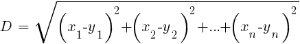
The algorithm simply predicts the target from the average k target variables of the nearest samples, weighted by their inverse distances. It can be used for both classification and regression. To predict the nearest neighbors, you can call the function knn in R or write your own C code for this purpose.
9. K-average
This is an approximation algorithm for uncontrolled classification. It is somewhat similar to the previous algorithm. To classify samples, the algorithm first places k random points in the function space. Then he assigns one of these points to all the samples with the shortest distance to it. The point then shifts to the average of these closest values. This generates new sample bindings, since some of them will now be closer to other points. The process is repeated until the re-binding as a result of the points shift stops, that is, until each point is average for the nearest samples. Now we have k sample classes, each located adjacent to some k-point.
This simple algorithm can produce surprisingly good results. In R, the kmeans function is used to implement it, an example of the algorithm can be found
by reference .
10. Naive Bayes
This algorithm uses the Bayesian theorem for the classification of samples of non-numeric functions (events), like the candlestick patterns mentioned above. Suppose event X (for example, the Open parameter of the previous bar is lower than the Open parameter of the current bar) appears in 80% of the winning samples. Then what is the probability of winning a sample if it has an X event? This is not 0.8 as you might think. This probability is calculated by the formula:
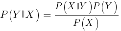
P (Y | X) is the probability that the event Y (profit) will occur in all samples containing event X (in our example, Open (1) <Open (0)). According to the formula, it equals the probability of an X occurring in all winning samples (in our case, 0.8) multiplied by the probability Y in all samples (approximately 0.5 if you follow the tips on balancing samples) and divided by the probability of occurrence of X in all samples
If we are naive and assume that all events X are independent of each other, then we can calculate the total probability that the sample will be winning by simply multiplying the probabilities P (X | winning) for each event X. Then we come to the following formula:
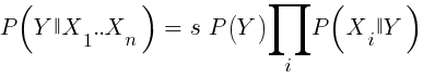
With the scaling factor s. For the formula to work, the functions must be chosen in such a way that they are as independent as possible. This will be an obstacle to the use of naive Bayes for trading. For example, two events Close (1) <Close (0) and Open (1) <Open (0) are not likely to be independent of each other. Numeric predictors can be converted to events by dividing the number into separate ranges. Naive Bayes is available in the e1071 package for R.
11. Decision and Regression Trees
Such trees predict the result of numerical values based on a yes / no decision chain in the tree branch structure. Each solution represents the presence or absence of events (in the case of non-numerical values) or comparison of values with a fixed threshold. A typical tree function generated by, for example, the Zorro framework looks like this:
int tree(double* sig) { if(sig[1] <= 12.938) { if(sig[0] <= 0.953) return -70; else { if(sig[2] <= 43) return 25; else { if(sig[3] <= 0.962) return -67; else return 15; } } } else { if(sig[3] <= 0.732) return -71; else { if(sig[1] > 30.61) return 27; else { if(sig[2] > 46) return 80; else return -62; } } } }
How does a tree come from a set of samples? There may be several methods for this, including
Shannon's informational entropy .
Decision trees can be quite widely used. For example, they are suitable for generating predictions that are more accurate than can be achieved using neural networks or support vectors. However, this is not a universal solution. The most famous algorithm of this type is C5.0, available in the C50 package for R.
To further improve the quality of predictions, you can use sets of trees — they are called a random forest. This algorithm is available in R packages called randomForest, ranger and Rborist.
Conclusion
There are many methods of data mining and machine learning. The critical question here is: what is better, model-based or machine-learning strategies? There is no doubt that machine learning has a number of advantages. For example, you do not need to take care of the microstructure of the market, the economy, take into account the philosophy of market participants or other similar things. You can concentrate on pure mathematics. Machine learning is a much more elegant and attractive way to create trading systems. On its side, all the advantages, except for one thing - in addition to stories on the forums of traders, the success of this method in real trading is problematic to track.
Almost every week there are new articles about trading using machine learning. Such materials should be taken with a fair amount of skepticism. The authors of some works claim fantastic winning rates of 70%, 80% or even 85%. At the same time, few people say that you can lose money even if the predictions are winning. An accuracy of 85% is usually translated into a profitability indicator above 5 - if everything were so simple, then the creators of such a system would have become billionaires. However, for some reason, to reproduce the same results, simply repeating the methods described in the articles, it does not work.
Compared to model-based systems, there are very few real successful machine learning systems. For example, they are rarely used by successful hedge funds. Perhaps in the future, when computing power becomes even more accessible, something will change, but so far deep learning algorithms remain a more interesting hobby for geeks than a real tool for making money on the exchange.
Other materials on finance and stock market from ITI Capital :