Last week, we figured out how the gait coordination algorithm of the legendary BigDog works. The robot was not yet autonomous and could cross the terrain only under the control of the operator.
Most of the readers last time approved the idea of a new translation - about how BigDog learned to independently navigate the way to the desired point and to orient in space. Well, actually, here it is. The BigDog navigation system uses a combination of planar laser scanning, stereo vision and proprioceptive perception. It is used to determine the location of the robot in the surrounding world. It detects obstacles and places them in a two-dimensional model of the world. Then she plans the way and controls the robot to follow the chosen trajectory. The path planner is a variation of the classic A * search algorithm. The smoothing algorithm processes the results obtained and transfers them to the path following algorithm. That one calculates the steering commands for BigDog.
The described system was tested in a forest zone with many trees, boulders, undergrowth. In addition to the flat areas, it also had slopes (up to 11 degrees). A total of 26 tests were performed, of which 88% were successful. The robot "saw" the terrain within a radius of 130 meters when driving at a given speed and traveled more than 1.1 km.
Equipment
1) Proprioceptive sensorsUsed to control BigDog gait and standalone navigation. Each of the 16 active and 4 passive degrees of freedom of the robot is equipped with a sensor. They provide current position and load data. This information is combined with IMU data to assess the state of contact with the ground, the height of the body position, the speed of the body. In addition, a number of sensors shows the state of the motor, computational, hydraulic, thermal and other BigDog systems.
Sensors BigDog: a) GPS-antenna; b) lidar; c) Bumblebee stereo camera; d) IMU from Honeywell; e) joint sensors.2) Exteroceptive SensorsThe robot is equipped with four external sensors: the SICK LMS 291 lidar, the PointGrey stereo camera from Bumblebee, the NovAtel GPS receiver and the Honeywell IMU. Data from them enter the system shown in the diagram below.
3) ComputersTo implement the system with the above scheme, two computers are used. The main computer BigDog - PC104 with a single-core Intel Pentium M processor (1.8 GHz). It interacts with proprioceptive sensors, controls the balance and movements of the robot, calculates the current model of the environment and the way through it, and also controls the gait.
Vision is provided by a separate computer on an Intel CoreDuo processor (1.7 GHz). It communicates with a pair of cameras, detects inconsistencies, evaluates visual odometry, and supports a 3D map of the area. This computer transmits the map and visual odometry data to the host computer with a frequency of 15 Hz via the onboard local area network.
The advantage of such a system is the ability to simplify the task of planning, breaking it into two parts. The data from the lidar and sensors are three-dimensional, but we can rely on the self-stabilization of the gait control system to abandon the more complex 3D perception and planning.
Technical approach
In our general technical approach, we use data from two environmental sensors to identify obstacles, calculate the trajectory of movement through or around obstacles, and command the control system of the robot’s gait to follow a given trajectory.
The whole process can be divided into three stages. First, images from the lidar and camera are processed to obtain a list of points indicating obstacles in the environment. Then these points are divided into non-intersecting objects and tracked for some time. Further, these objects are combined in a temporary memory for making a cartogram. This cartogram is used to plan the direction of movement towards an intermediate goal. The scheduler is designed to control that the BigDog trajectories are at a proper distance from obstacles and that the trajectories are stable in space during the iterations of the scheduler. The motion algorithm for a given trajectory forces the robot to follow the intended path by sending speed commands to the gait control system. That one moves the limbs of the robot in turn.
A. Information Collection
1) Assessment of the situationThere are two sources of odometric information: kinematic sensors in the legs and an artificial vision system. The data obtained from them are combined to assess the location of the robot.
The odometer system uses the kinematic information obtained from the legs to calculate the movements of the robot. A visual odometry system tracks visual characteristics to calculate movement. Both of these tools use an inertial measurement module (IMU) as a source of information for spatial orientation. The general calculator combines the output of these two odometers, focusing on visual odometry at low speeds and kinematics at higher speeds. Combining these two indicators eliminates the shortcomings of each of the calculators: the possible failure of stereo systems, the odometer drift, located in the limbs, while running in place, as well as the sensor's error along the vertical axis.
The lidar used in the BigDog robot produces a new image every 13 milliseconds. Each image is transformed into an external coordinate system with the center at the location of the robot. This uses time-synchronized information from the location calculator. The resulting 3D point cloud is then transmitted to the segmentation algorithm described below for processing. Similarly, the stereoscopic vision system collects discrepancy maps for some time to create a 3D map of the area in a 4 x 4 meter square centered on the robot. The spatial filter determines areas of significant height variation (i.e., potential obstacles) and transmits a list of points belonging to these areas to the point cloud segmentation algorithm.
2) Point cloud segmentation and object trackingDue to the irregularities of the earth and the movements of the robot, part of the lidar-scanner data will include images of the earth. Reflections from long obstacles (for example, walls) are similar in appearance to reflections from the earth's surface. For successful operation, the system must interpret these reflections so that it can control the robot near the walls, and not “fear” the earth. The first step in this process is the segmentation of the obstacle points provided by the lidar and the terrain map into separate objects. Rare 3D clouds of points are segmented into objects by merging individual points separated by a distance of less than 0.5 meters.
Objects obtained by the segmentation algorithm are tracked for some time. To accomplish this task, we use a greedy iterative algorithm with heuristic constraints. The object in the current image coincides with the nearest object of the last image, provided that the objects are separated by a distance of no more than 0.7 meters.
Due to the fact that point clouds are segmented into objects and tracked for some time, the robot can adequately move in an environment with moderate unevenness of the earth and obstacles of various kinds: trees, cobblestones, fallen logs, walls. Trees and walls are determined mainly by a lidar scanner, and cobblestones and logs are determined by a stereoscopic vision system.
A sequence of illustrations showing a robot (yellow box) with: a) data from a lidar (blue dots) recorded in a few seconds; b) their respective objects. Tall brown objects are trees. Reflections from the ground are transparent and flat. A green cylinder is a goal; the blue line of the calculated path leads to it. c) Top view of the cartogram: the areas with the lowest lethal value are green, the areas with the highest such value are mauve. Each unit of the grid corresponds to 5 meters.B. Planning navigation
Our approach to solving the problem of navigation is common in the robotic community. Obstacle points (obtained through perceptual processes) are plotted on a cartogram centered on the location of the robot. The ultimate goal of the robot is projected onto the border of the cartogram, and the variant of algorithm A ∗ is applied to it. This process is repeated about once per second.
1) Tracked obstacle memoryDue to the limited field of view of the two sensors of the robot, it is extremely important that the robot maintains an accurate memory of the obstacles that it can no longer see. Since the list of objects is provided by the object tracking system, individual objects are added, updated, or deleted in the object memory of the planning system. The size of the list of objects is limited, so when adding new objects to it, others should be deleted.
Denoting the current list of objects with the variable O, we can calculate two parameterized subclasses of O:
Here age (q) is the difference between the current time and the last measurement time of the object q,
norm (q, r) inf is the minimum distance between the current location of the robot and the boundary of the object q.
Objects are removed from O by the following criteria:- The set {P (30) ∩ Q (15)} is subtracted from O. These are objects older than 30 seconds and located no closer than 15 meters to the robot.
- The set {P (1800) ∩ Q (10)} is subtracted from O. These are objects older than half an hour and located no closer than 10 meters to the robot.
- Objects are removed from O as they reach the list limit. The priority of an object is determined by the time during which it was successfully tracked by the tracker. In other words, objects that the robot has “watched” for longer are stored in memory longer.
- However, no object tracked in the previous 10 seconds is discarded.
Such a distribution of memory resources leads to the following behavior: as the objects leave the field of view of the sensors of the robot, it forgets remote objects and objects that it has not seen several times. Objects that are in sight or inaccessible, but located close to the robot, are not forgotten.
2) Creating cartogramsWe use a cartogram based on a 2D grid to represent the environment around the robot. Instead of dynamically composing a cartogram (as the robot receives new information about the environment), a new cartogram is compiled with each planning iteration and filled with objects from the memory of the scheduler. From this it follows that the dynamic route planner cannot be used instead of the A * algorithm. Since we assume that the size of the objects is limited (that there is no dead end in the environment more than half the map), the scope of the planning task and the time to calculate the path are small.
The cartogram is filled with values from the list of objects in accordance with the following algorithm:
Cells where objects are located are assigned a very high lethal value. The indicator for cells in the vicinity of the object is set in accordance with the function f, which takes into account the current distance to this point. For the test results presented here, f was simply the inverse of the distance cube.
The effect of this approach is that from cells with a very high value, it decreases gradually as they move away from them (and the objects they designate).
3) Road stabilityTo ensure that we are not “managing” BigDog in a random and haphazard manner, special attention is paid to the sustainability of the planned path. It should be as stable as possible in the iterations of the path planner. This is provided in three ways.
First, the starting point transmitted to the algorithm A * is not the current position of the robot, but the projection of its position at the end point of the path, previously issued by the algorithm A * (let's call this point p). While BigDog follows the planned path, it may deviate slightly from it to the side. Projecting the starting point to the point of the previous calculation of the A * algorithm, we filter out the oscillation of the robot position, and the paths that the scheduler displays become more stable. If the robot deviates from the path more than the set value (by default it is 3 meters), the point p is simply transferred to the current position of the robot.
Secondly, to ensure the continuity of the path planner, we calculate q - the projection of the robot position from 2.5 seconds in the past to the last point calculated by algorithm A *. Then the segment of the last planned path from q to p is added to the calculation of the new path. As a result, the robot tracks a short distance already traveled. Due to this, the algorithm of following the path shows itself better in case of significant violations of the situation, which are often encountered by robots on their feet.
Thirdly, some history of planned paths is stored in the memory of the robot. These paths are used to reduce the values of those cells of the cartogram, where the robot has already gone, with a simultaneous increase in the value of the cells of the surrounding area. Therefore, as a rule, the new planned path in the same direction will repeat the path already passed by the robot (but without a strict guarantee of this).
4) Smoothing the pathThe computed path, since it is based on a regular grid, is slightly jagged. Significant changes in direction can cause unwanted control commands. To avoid this, a DeBur smoothing algorithm is applied.
In addition, planning paths based on the grid often leads to technically optimal, but less desirable paths to the goal. We solve this problem by calculating the smoothed path for each iteration of the scheduler. For subsequent iterations, the cells of the map, where the smoothed path runs, are assigned a smaller value. This provides a more direct and smooth path to the goal.
C. Gait Control: Mobility and Balance
The navigation planning system determines the new path about once per second. The path-following algorithm, which operates at a frequency of 200 Hz, guides the robot in accordance with the last planned path. This algorithm creates a set of commands in the form of the desired body speeds, including forward speed, lateral speed and body yaw rate. These speeds are transmitted to the gait controller, which controls the movement of the legs.
Based on the distance between the robot and the path, one of three strategies is used. If the robot is located close to the section of the path, it begins to move diagonally until it reaches it from the side, moving at full speed. If the robot is far from the path, it is directed straight ahead to the desired point. In the intermediate position, a combination of these strategies is used.
A detailed description of gait control algorithms is beyond the scope of this article. However, as a rule, body speeds act as control inputs for low-level BigDog gait controllers. The gait controller produces commands of force and position for each joint to ensure stability, reacts to disturbances and provides the body with the necessary speeds. Although the calculations of the path investigator’s algorithm can be used for any BigDog gait, the trot gait is optimal due to the speed and possibility of crossing rough terrain.
Field Test Results
The sensor and navigation system described above was installed on BigDog and tested outside the laboratory. The tests were conducted on the ground, where there were many trees, boulders, undergrowth, hills with slopes up to 11 degrees. Figure 1 shows examples of the landscape. Figure 2 shows the data from the lidar processed by the robot.
Fig. 1. Landscape of the area where the tests were conductedFig. 2. Test tests, top view. The image was obtained from the lidar and stereo cameras. Dark areas - trees and other obstacles. The size of the grid is 5 meters.The navigation system and the scheduler were developed for 7 months, with regular tests about once every five weeks. Here are the results of recent tests.
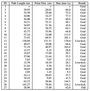
Of the 26 tests conducted, 23 ended successfully: the robot reached the goal, did not encounter any of the obstacles, and was not close to it. The outcomes of these tests are marked in the pivot table as Goal (“Target”). The robot fell at the end of only one test after stepping on a small stone. Usually the gait control system copes with such situations, but not this time (the result is noted in the table as Fall - “Fall”). In the three tests, the robot encountered large obstacles on its way (more than 20 meters wide). The robot calculated from which side it is better to bypass the obstacle and did not make progress in a given period of time (20 seconds). Obstacles of this size are beyond the scope for which the autonomous system was developed. The results of these tests in the table are labeled Live-lock ("Lock").
In these 26 tests, the robot was placed in fairly similar scenarios and forest terrain of the middle zone. With the increasing complexity of the environment, the number of outcomes of Live-lock increases, and the robot selects less efficient paths.
More interesting - on robo-hunter.com :
Our YouTube channel